1

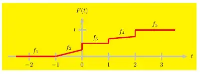
Consider the following example from this answer:

\documentclass[border=0bp]{standalone}

\usepackage{pst-plot}

\begin{document}

\psset{unit=1.5cm} \begin{pspicture}showgrid=false(4,2) \psframe*linecolor=yellow,opacity=0.5(4,2) \psaxes[linecolor=lightgray]{->}(0,0)(-2.5,-0.5)(3.5,1.5)[$t$,0][$F(t)$,90] \psset{algebraic,linewidth=1.5pt,linecolor=red} \pscustom { \psplot{-2.5}{-1}{0} \psplot{-1}{0}{(x+1)/4} \psplot{0}{1}{1/2} \psplot{1}{2}{(x+7)/12} \psplot{2}{3.5}{1} } \end{pspicture}

\end{document}

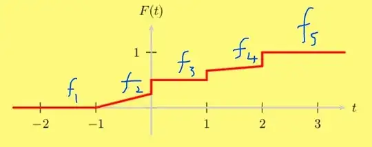
I wonder how I could add labels to each piece of this piecewise function so that it look like this $f_1$ to $f_5$

It would be great if I could adjust the coordinate of those labels freely. A stupid way is that I can add a "transparent" point to a certain coordinate of the figure and add a label to that point, but I don't even know how to do this.
enter image description here

No One
  • 269

2 Answers2

1
\documentclass[border=0bp]{standalone}

\usepackage{pst-plot}

\begin{document}

    \psset{unit=1.5cm}
    \begin{pspicture}[showgrid=false](-2.75,-0.75)(4,2)
        \psframe*[linecolor=yellow,opacity=0.5](-2.75,-0.75)(4,2)
        \psaxes[linecolor=lightgray]{->}(0,0)(-2.5,-0.5)(3.5,1.5)[$t$,0][$F(t)$,90]
        \psset{algebraic,linewidth=1.5pt,linecolor=red}
        \pscustom
        {
            \psplot{-2.5}{-1}{0}
            \psplot{-1}{0}{(x+1)/4}
            \psplot{0}{1}{1/2}
            \psplot{1}{2}{(x+7)/12}
            \psplot{2}{3.5}{1}
        }
        \pcline[linestyle=none](-2.5,0)(-1,0)\naput{$f_1$}
        \pcline[linestyle=none](-1,0)(0,0.25)\naput{$f_2$}
        \pcline[linestyle=none](0,0.5)(1,0.5)\naput{$f_3$}
        \pcline[linestyle=none](1,0.67)(2,0.75)\naput{$f_4$}
        \pcline[linestyle=none](2,1)(3.5,1)\naput{$f_5$}
    \end{pspicture}

\end{document}

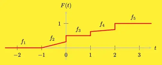
enter image description here

For this simple example it would make sense to define the nine points and then using a \psline.

\documentclass[border=0bp]{standalone}
\usepackage{pst-plot}
\begin{document}
\psset{unit=1.5cm}
\begin{pspicture}[showgrid=false](-2.75,-0.75)(4,2)
    \psframe*[linecolor=yellow,opacity=0.5](-2.75,-0.75)(4,2)
    \psaxes[linecolor=lightgray]{->}(0,0)(-2.5,-0.5)(3.5,1.5)[$t$,0][$F(t)$,90]
    \psset{algebraic,linewidth=1.5pt,linecolor=red}
    \pnodes{A}(-2.5,0)(-1,0)(-1,0)(0,0.25)(0,0.5)(1,0.5)(1,0.67)(2,0.75)(2,1)(3.5,1)
    \multido{\iA=0+2,\iB=1+2,\iC=2+2,\iD=1+1}{5}{%
      \pcline(A\iA)(A\iB)\naput{$f_\iD$}
        \ifnum\iA<7 \psline(A\iB)(A\iB|A\iC)\fi}
\end{pspicture}

\end{document}

user187802
  • 16,850
  • Sorry for this stupid question , but what is the meaning of (1,0.67)(2,0.75) in the code \pclinelinestyle=none(2,0.75)\naput{$f_4$}? I thought I only need one coordinate for the label, so why are there two of them? And how do they together determine the position of $f_1$? – No One Sep 30 '22 at 19:01
  • That are the start and endpoint of the functions and with \pcline it will be converted to nodes, which can be used automatically by \naput (node above) – user187802 Sep 30 '22 at 19:10
0

Consider also the less exotic tikz code:

\documentclass{article}
\usepackage{tikz}

\begin{document} \begin{tikzpicture}[scale=1.5,line width=2pt] \filldraw[yellow] (-3,-.5) rectangle (4.3,2); \draw[gray!50,-latex] (-2.8,0)--(4,0) node[black,right] () {$t$}; \draw[gray!50,-latex] (0,-0.15)--(0,1.5) node[black,above] () {$F(t)$}; \foreach \i in {-2,-1,...,3} \draw[gray!50] (\i,.15)--(\i,-.15) node[black,below] () {$\i$ }; \draw[gray!50] (.15,1)--(-.15,1) node[black,left] () {$1$ }; \draw[red] (-2.5,0)--(-1,0) node[pos=.5,above,black] () {$f_1$}; \draw[red] (-1,0)--(0,.25) node[pos=.5,above,black] () {$f_2$}; \draw[red] (0,.25)--(0,.5); \draw[red] (0,.5)--(1,.5) node[pos=.5,above,black] () {$f_3$}; \draw[red] (1,.5)--(1,.67); \draw[red] (1,.67)--(2,.75) node[pos=.5,above,black] () {$f_4$}; \draw[red] (2,.75)--(2,1); \draw[red] (2,1)--(3.5,1) node[pos=.5,above,black] () {$f_5$}; \end{tikzpicture} \end{document}

with this output:

enter image description here