Your images are to wide that can be fit in one column width. There in the case, that images had to be placed in one column, is beside
- reducing font size to
\small or even to \footnotesie,
- reducing width of nodes with allowing multi lines text in them,
- reducing horizontal distances between modes,
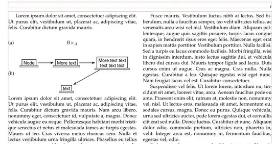
not much possibilities to what can be done. An example how aforementioned can be implemented is:
\documentclass[10pt,journal,compsoc]{IEEEtran}
\usepackage{lipsum}
%---------------- show page layout. don't use in a real document!
\usepackage{showframe}
\renewcommand\ShowFrameLinethickness{0.15pt}
\renewcommand*\ShowFrameColor{\color{red}}
%---------------------------------------------------------------%
\usepackage{lipsum}
\usepackage{amsmath}
\makeatletter
\newcommand{\leqnos}{\tagsleft@true\let\veqno\@@leqno}
\newcommand{\reqnos}{\tagsleft@false\let\veqno\@@eqno}
\reqnos
\makeatother
\usepackage{tikz-cd}
\usetikzlibrary{arrows.meta,
                positioning}
\begin{document}
\lipsum[1][1-3]
\begingroup\leqnos
\begin{equation}
   \begin{tikzcd}
       B\times_A
   \end{tikzcd}~\tag{a}
\end{equation}
\begin{equation}
    \begin{tikzpicture}[baseline=(current bounding box.center),
 node distance = 13mm,
compute/.style = {draw, thick, font=\small\sffamily, align=center,
                  append after command={\pgfextra{\let\LN\tikzlastnode}
                    (\LN.south west) edge[double=gray!50,double distance=3pt,
                                          line cap=rect,
                                          shorten >=-2pt,shorten <=-2pt]
                    (\LN.south east)}},
                        ]
    \node[compute] (n1) {Node};
    \node[compute,right=of n1] (n2) {More text};
    \node[compute,right=of n2] (n3) {More text text\ text text text};
    \node[compute,below=of n2] (n4) {text};
    \draw[thick,draw, -Stealth, shorten > = 3pt, shorten < = 3pt]
        (n1) edge (n2)
        (n2) edge (n3)
        (n3) to (n4);
   \end{tikzpicture}~\tag{b}
\end{equation}
   \endgroup
\lipsum
\end{document}
Addendum:
From comment follows:
- in you approach is not possible to obtain what you after
- one way is to define new environment, which has )not referable) tag on the left, and images or other text on the right, centered or raggedleft.
- example of sucn command can be:
\usepackage{tabularray}
\newcommand\LST[3]{
    \begin{center}
    \begin{tblr}{colspec={@{} Q[c, font=\bfseries] X[#1] @{}} }
    #2  &   #3

    \end{tblr}
    \end{center}}
- In use of above definition you need to a wee bit to redefine
compute node style:
compute/.style = {draw, thick, font=\small\sffamily, align=center,
                  append after command={\pgfextra{\let\LN\tikzlastnode}
                    ([xshift=-2pt] \LN.south west)
                        edge[double=gray!50,double distance=3pt,
                                          line cap=rect]
                    ([xshift=+2pt] \LN.south east)}},
                        ]
- An exampe, how to use aforementioned, is:
\documentclass[journal,compsoc]{IEEEtran}
\usepackage{tabularray}
\newcommand\LST[3]{
    \begin{center}
    \begin{tblr}{colspec={@{} Q[c, font=\bfseries] X[#1] @{}} }
    #2  &   #3
    \end{tblr}
    \end{center}}
\usepackage{caption}
\usepackage[export]{adjustbox}
\usepackage[label font=bf, labelformat=simple]{subfig}
\usepackage{lipsum}
\usepackage{tikz-cd}
\usetikzlibrary{arrows.meta,
                positioning}
\begin{document}
\lipsum[1][1-3]
\LST{c}{(a)}{$B\times_A$}
\LST{r}{(b)}{%
\begin{tikzpicture}[baseline=(current bounding box.center),
 node distance = 12mm,
compute/.style = {draw, thick, font=\small\sffamily, align=center,
                  append after command={\pgfextra{\let\LN\tikzlastnode}
                    ([xshift=-2pt] \LN.south west)
                        edge[double=gray!50,double distance=3pt,
                                          line cap=rect]
                    ([xshift=+2pt] \LN.south east)}},
                        ]
    \node[compute] (n1) {Node};
    \node[compute,right=of n1] (n2) {More text};
    \node[compute,right=of n2] (n3) {More text text\ text text text};
    \node[compute,below=of n2] (n4) {text};
    \draw[thick,draw, -Stealth, shorten > = 3pt, shorten < = 3pt]
        (n1) edge (n2)
        (n2) edge (n3)
        (n3) to (n4);
   \end{tikzpicture}%
        }
\lipsum
\end{document}
Sorry, due to (github) server error I cant upload image produce with above MWE.


