Strange syntax in pgfplot

Question

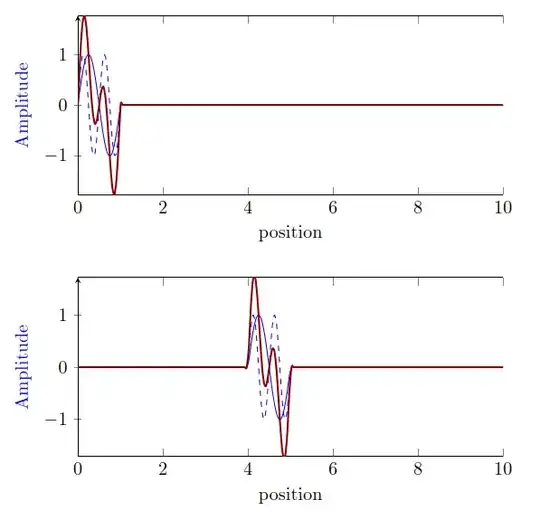
I want to display propagation of a signal, obtained as addition of 2. It works as I want writing:

\documentclass{standalone}
\usepackage[usenames,svgnames]{xcolor}
\usepackage{siunitx}
\usepackage{tikzscale}
\usepackage{pgf,tikz,pgfplots}
\usetikzlibrary{math}
\begin{document}
     \begin{tikzpicture}
       \tikzmath{
       \omm=0;
       \omM=10;
       % sin sur une période, 0 sinon
       function sina(\x) {
        if and(\x>0,\x<1) then { 
       return sin(360\x);}
        else {return 0;};};
       % fréquence double
       function sinb(\x) {
        if and(\x>0,\x<1) then { 
       return sin(720\x);}
        else {return 0;};};
       }
   \begin{axis}[width=.8\columnwidth,
   height=5cm,
   xmin=\omm,
   xmax=\omM,
   axis y line=left,
   ylabel= \textcolor{blue}{Amplitude},
   xlabel= position,
    smooth,
   ]
   \addplot+[blue,thin, mark=none, samples=200,domain = \omm:\omM] {sina(x)};
   \addplot+[blue,thin, dashed, mark=none, samples=200,domain = \omm:\omM] {sinb(x)};
   \addplot+[DarkRed,thick, mark=none, samples=200,domain = \omm:\omM] {sina(x)+sinb(x)};
   \end{axis}
   \begin{axis}[width=.8\columnwidth,
   height=5cm,
   yshift=-5cm,
   xmin=\omm,
   xmax=\omM,
   axis y line=left,
   ylabel= \textcolor{blue}{Amplitude},
   xlabel= position,
    smooth,
   ]
   \addplot[blue,thin, mark=none, samples=200,domain = \omm:\omM] {sina(x-4)};
   \addplot[blue,thin, dashed, mark=none, samples=200,domain = \omm:\omM] {sinb(x-4)};
   \addplot+[DarkRed,thick, mark=none, samples=200,domain = \omm:\omM] {sina(x-4)+sinb(x)};
   \end{axis}
 \end{tikzpicture}

\end{document}

but I definitively wouldn't expect to write sina(x-4)+sinb(x) for the shifted addition, but sina(x-4)+sinb(x-4)...

Is it really the expected behavior? If it is, can the logic behind be explained, as I found the good syntaxe by mistake.

Edit: Another alternative syntax to get the correct result, maybe it can help someone to understand what's happening:

\addplot+[DarkRed,thick, mark=none, samples=200,domain = \omm:\omM] {sinb(\x-4) + sina(\x-4)};

Replacing the usual x variable in the \addplot syntax for functions by \x shifts as expected the function sina.

Edit 2: If in the definition of sina() or sinb() the name of the variable is changed, for example by \y, the expected behavior is back. By replacing the definition of sinb() by:

% fréquence double
       function sinb(\y) {
        if and(\y>0,\y<1) then {
       return sin(720*\y);}
        else {return 0;};};

then the expected syntax (sina(x-4)+sinb(x-4) ) gives the expected result.

If you have problems when summing sines, then you should ask on a math forum — hpekristiansen, Oct 28 '22 at 05:32
Note that you test for 0 > (x - 4) > 1 in your functions, so x ≠ \x in the second example. If you use, for example, (x - 1) as \x, you get sin(360x + 360) for the first function and sin(720x + 720) for the second function. Thus, the second function returns a result that is shifted relative to the first one. Since you only add the parts from the functions where 0 > (x - 1) > 1, these two parts will never overlap. At least to my humble understanding ... — Jasper Habicht, Oct 28 '22 at 06:55
What I want to illustrate is propagation of a signal, f(x-ct) with or without dispersion in a linear medium (sin wave propagating at different speed in the dispersive case). So it's ok to test for $0 > (x - 4) > 1$ in the second case for both "si during a time unit" functions, as i want the signal between 4 and 5, and 0 everywhere else (non dispersive case, both sin move at the same speed). That's what I obtained in the almost MWE, but I don't understand why the sinb function is shifted in the working-but-i-dont-understand-why syntax, as it as x as argument, and not x-4 as I expect. — Hérisson Didier, Oct 29 '22 at 01:34
Related question: https://tex.stackexchange.com/questions/611793/pgfplots-x-vs-x, which is not entirely conclusive but it seems to suggest that x and \x are intended to be the same (so if they are not the same then something strange is going on). — Marijn, Nov 09 '22 at 19:42
@Marijn Thank you. I added a comment to this question as an example where they don't behave the same. A colleague found another workaround, by changing the name of the variable I'm using by default, x in the definitions of functions. — Hérisson Didier, Nov 09 '22 at 20:29

schtandard · Accepted Answer · 2022-11-12T15:56:08.650

This is definitely a bug. The argument of sina is assigned to \x internally (if you used that name in the definition) and this value seems to leak out to the sinb call. That is, the second call behaves as if x were the entire argument of the first call. As you already noticed, this strangely does not happen when using \x instead of x. I do not understand the reason for this behavior, but it is definitely a bug, so I reported it.

I can, however, suggest an alternative: Use declare function instead of \tikzmath. It is recommended in the pgfplots manual as a best practice for conserving compatibility with the lua backend (as illustrated in this answer), which gives you more accuracy and speed, and offers all of the functionality you need, I think. Importantly, it does not exhibit the same bug:

\documentclass{article}
\usepackage[usenames,svgnames]{xcolor}
\usepackage{pgfplots}
\pgfplotsset{compat=1.18}
\begin{document}
\begin{tikzpicture} [
      declare function={
        ommin = 0;
        ommax = 10;
        sina(\x) = ifthenelse(and(\x>0, \x<1), sin(360x), 0);
        sinb(\x) = ifthenelse(and(\x>0, \x<1), sin(720x), 0);
%        % or, a bit more compactly:
%        sina(\x) = (0<\x && \x<1 ? sin(360\x) : 0);
%        sinb(\x) = (0<\x && \x<1 ? sin(720\x) : 0);
      },
    ]
  \begin{axis}[width=.8\columnwidth,
      height=5cm,
      xmin=ommin,
      xmax=ommax,
      axis y line=left,
      ylabel= \textcolor{blue}{Amplitude},
      xlabel= position,
      smooth,
    ]
  \addplot+[blue,thin, mark=none, samples=200,domain=ommin:ommax] {sina(x)};
  \addplot+[blue,thin, dashed, mark=none, samples=200,domain=ommin:ommax] {sinb(x)};
  \addplot+[DarkRed,thick, mark=none, samples=200,domain=ommin:ommax] {sina(x)+sinb(x)};
  \end{axis}
  \begin{axis}[width=.8\columnwidth,
      height=5cm,
      yshift=-5cm,
      xmin=ommin,
      xmax=ommax,
      axis y line=left,
      ylabel= \textcolor{blue}{Amplitude},
      xlabel= position,
      smooth,
    ]
  \addplot+[blue,thin, mark=none, samples=200,domain=ommin:ommax] {sina(x-4)};
  \addplot+[blue,thin, dashed, mark=none, samples=200,domain=ommin:ommax] {sinb(x-4)};
  \addplot+[DarkRed,thick, mark=none, samples=200,domain=ommin:ommax] {sina(x-4)+sinb(x-4)};
  \end{axis}
\end{tikzpicture}
\end{document}

@Dr.ManuelKuehner Always nice, when there are related bountied quesions. ;-) — schtandard, Nov 12 '22 at 09:17
Thanks for your answer. It would be nice if you could fill a bug report on the github project page. — cjorssen, Nov 12 '22 at 12:36
@cjorssen As I wrote (and linked) in my answer, I did report this. I wasn't sure at first if it belonged to pgfplots or pgf, since it seemed to be a \tikzmath problem but I somehow couldn't reproduce it without \pgfplots. I went with the latter in the end and it seems to be correct. (Someone else reproduced it without pgfplots, don't know why I didn't get there.) — schtandard, Nov 12 '22 at 15:48
@schtandard Thanks a lot. Sorry I missed you mentioned you reported the bug :-) — cjorssen, Nov 13 '22 at 14:34
Thank you for the report and great explanation, I learned more than expected! happy to validate the bounty. — Hérisson Didier, Nov 13 '22 at 22:01

Strange syntax in pgfplot

1 Answers1

Linked