1

I am trying to replicate this excellent answer which explains how to draw Brownian motions in TiKZ:

\newcommand{\Lathrop}[6]{% points, advance, rand factor, options, end label, truncate from point
    \draw[#4] (0,0)
    \foreach \x in {1,...,#6} { 
        -- ++ (#2,rand*#3)
    }
    coordinate (tempcoord) {};
    \pgfmathsetmacro{\remainingwidth}{(#1-#6)*#2}; % changed to a custom number
    \def\remainingwidthcustom{1};
    \draw[#4] (tempcoord) -- ++ (\remainingwidthcustom,0) node[right] {#5};
}

\begin{tikzpicture} \def\ylength{3} \pgfmathsetseed{3} % control pseudo-random number

% Axis
\coordinate (y) at (0,3); \coordinate (x) at (6,0);
\draw[<->] (y) node[above] {$S$} -- (0,0) --  (x) node[right] {$\mathbb{N}$};

% Brownian motion
\Lathrop{750}{0.02}{0.21}{blue!70!black}{strike price $S_N$}{250};

\end{tikzpicture}

My problem is that I cannot change it to the geometric Brownian motion for two reasons:

  1. I cannot get exponential function via pgfmathparse
  2. I do not fully understand the syntax inside the \foreach \x-loop.

Any help is appreciated.
qarabala
  • 202
  • 1
  • 9

1 Answers1

2

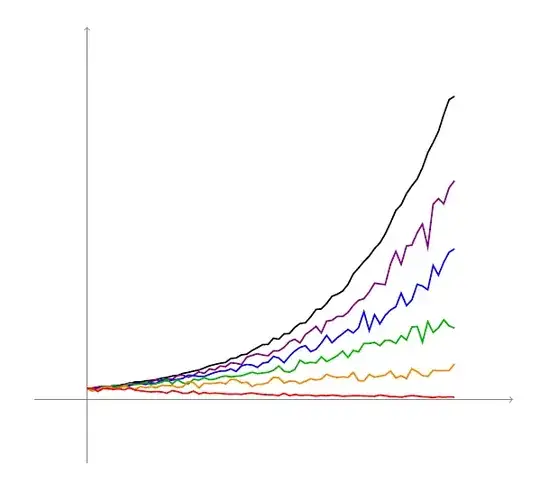
enter image description here

I used the function defined by Mark Wibrow (see Gaussian random numbers) to obtain a Gaussian random number and then draw the geometric Gaussian motions with different variance values based on those Gaussian random numbers.

The code

\documentclass[11pt, margin=.5cm]{standalone}
\usepackage{tikz}
\usetikzlibrary{math}

%% Mark Wibrow's code \newcount\gaussF \edef\gaussR{0} \edef\gaussA{0}

\makeatletter \pgfmathdeclarefunction{gaussR}{0}{% \global\advance\gaussF by 1\relax \ifodd\gaussF \pgfmathrnd@% \ifdim\pgfmathresult pt=0.0pt\relax% \def\pgfmathresult{0.00001}% \fi \pgfmathln@{\pgfmathresult}% \pgfmathmultiply@{-2}{\pgfmathresult}% \pgfmathsqrt@{\pgfmathresult}% \global\let\gaussR=\pgfmathresult%radius \pgfmathrnd@% \pgfmathmultiply@{360}{\pgfmathresult}% \global\let\gaussA=\pgfmathresult%angle \pgfmathcos@{\pgfmathresult}% \pgfmathmultiply@{\pgfmathresult}{\gaussR}% \else \pgfmathsin@{\gaussA}% \pgfmathmultiply@{\gaussR}{\pgfmathresult}% \fi }

\pgfmathdeclarefunction{invgauss}{2}{% \pgfmathln{#1}% <- might need parsing \pgfmathmultiply@{\pgfmathresult}{-2}% \pgfmathsqrt@{\pgfmathresult}% \let@radius=\pgfmathresult% \pgfmathmultiply{6.28318531}{#2}% <- might need parsing \pgfmathdeg@{\pgfmathresult}% \pgfmathcos@{\pgfmathresult}% \pgfmathmultiply@{\pgfmathresult}{@radius}% }

\pgfmathdeclarefunction{randnormal}{0}{% \pgfmathrnd@ \ifdim\pgfmathresult pt=0.0pt\relax% \def\pgfmathresult{0.00001}% \fi% \let@tmp=\pgfmathresult% \pgfmathrnd@% \ifdim\pgfmathresult pt=0.0pt\relax% \def\pgfmathresult{0.00001}% \fi \pgfmathinvgauss@{\pgfmathresult}{@tmp}% }

\begin{document} \tikzmath{% real \m, \s, \xBound, \yBound, \v0; \xBound = 3.5; \yBound = 7; \m = 1; \v0 = .2; function GBM(\t, \ini, \s) { % argument, initial value, standard deviation return {\iniexp((\m -\s\s/2)\t +\srandnormal/10))}; }; } \begin{tikzpicture}[xscale=2] \draw[gray, ->] (-.5, 0) -- (\xBound +.5, 0); \draw[gray, ->] (0, -1.2) -- (0, \yBound);

\foreach \s/\rgb in {.2/black, .5/violet, .7/blue, .9/green!70!black, 1.2/orange, 1.7/red}{% \draw[\rgb, thick] (0, \v0) \foreach \t in {.05, .1, ..., \xBound}{% -- (\t, {GBM(\t, \v0, \s)}) }; } \end{tikzpicture}

\end{document}

Daniel N
  • 5,687