Drawing a Flowchart for a Degree Plan

Question

I am new to drawing flowcharts using tikz. I need to draw a flowchart similar to the following one:

However, I could not get elbow arrows. I need to get elbow arrows that do not intersect the other rectangles. Here is my try.

This is the code. Please help me with the easiest way to draw such a flowchart.

\documentclass{article}
\usepackage{tikz}
\usetikzlibrary{shapes.geometric, arrows}
\usetikzlibrary{matrix,shapes,positioning,chains}
\tikzstyle{course} = [rectangle, rounded corners, 
minimum width=2cm, 
minimum height=1cm,
text centered, 
draw=black, 
fill=white!30]
\tikzstyle{arrow} = [thick,->,>=stealth]
\begin{document}
\begin{tikzpicture}[node distance=3cm]
% Freshman
\node (CHEM101) [course] {CHEM 101};
\node (ENGL101) [course, right of=CHEM101] {ENGL 101};
\node (MATH101) [course, right of=ENGL101] {MATH 101};
\node (PHYS101) [course, right of=MATH101] {PHYS 101};
\node (PE101) [course, right of=PHYS101] {PE 101};
\node (ENGL102) [course, below of=CHEM101] {ENGL 102};
\draw [arrow] (ENGL101) -- (ENGL102);
\end{tikzpicture}
\end{document}

Answer 1

You can use a matrix to position the nodes. And then you can define some macros that draw the connections. The macro implemented here tests wether the arrows are horizontal or vertical, and chooses the color accordingly. For vertical arrows, it allows you to shift the point at which the arrow attaches to the upper node (start shift), lower node (target shift) as well as an overall shift of both (shift). With nudge you can nudge the corner point of such arrows. It also allows you to avoid some nodes, and "intelligently" chooses the path either left or right of the avoided nodes. In the matrix, the nodes have names m-<row>-<column>, and column 1 is taken by the semesters. The syntax of the \Arrow command is

\Arrow[<options>]{<start>}{<target>}

where the start and target are given by <row>-<column>, but the avoided nodes have to be entered as (m-<row>-<column>). It is almost certainly the case that the macro does not allow you to do everything you end up wanting it to do, but you can upgrade it by adding some more options.

\documentclass[tikz,border=2mm]{standalone}
\usetikzlibrary{calc,fit,matrix}
\begin{document}
\begin{tikzpicture}[Arrow/.cd,start shift/.initial=0pt,target shift/.initial=0pt,% 
    shift/.initial=0pt,% overall shift
    nudge/.initial={(0pt,0pt)},
    avoid/.code=\ArrowAvoidtrue\def\ArrowAvoidnodes{#1},
    sep/.initial=1ex,
    /tikz/.cd,vc/.style={thick,blue!80,-stealth,rounded corners=0.5pt},
    hc/.style={thick,orange,-stealth,rounded corners=0.5pt}    
    ]
 \newif\ifArrowAvoid
 \newcommand{\Arrow}[3][]{\begingroup\ArrowAvoidfalse   
    \tikzset{Arrow/.cd,#1}%
    \ifArrowAvoid
     \node[fit=\ArrowAvoidnodes,inner sep=\pgfkeysvalueof{/tikz/Arrow/sep}](Avoid){};
     \draw[vc] let 
        \p1=(Avoid),
        \p2=([xshift=\pgfkeysvalueof{/tikz/Arrow/shift}+\pgfkeysvalueof{/tikz/Arrow/start shift}]m-#2.south),
        \p3=([xshift=\pgfkeysvalueof{/tikz/Arrow/shift}+\pgfkeysvalueof{/tikz/Arrow/target shift}]m-#3.north),
        \n1={int(scalar(ifthenelse(0.5*\x2+0.5*\x3>\x1,1,0)))} in 
        \ifcase\n1\relax 
            (\p2) |- (Avoid.north west) -- (Avoid.south west) -| (\p3)
        \or 
            (\p2) |- (Avoid.north east) -- (Avoid.south east) -| (\p3)
        \fi; 
    \else 
     \draw let \p1=($(m-#3)-(m-#2)$) in 
        \ifdim\y1=0pt\relax 
         [hc] (m-#2) -- (m-#3)
        \else 
        let \p2=([xshift=\pgfkeysvalueof{/tikz/Arrow/shift}+\pgfkeysvalueof{/tikz/Arrow/start shift}]m-#2.south),
            \p3=([xshift=\pgfkeysvalueof{/tikz/Arrow/shift}+\pgfkeysvalueof{/tikz/Arrow/target shift}]m-#3.north),
            \p4=\pgfkeysvalueof{/tikz/Arrow/nudge},
            \n1={int(ifthenelse(\x1==\x2,0,1))} in 
            \ifcase\n1\relax
                [vc] (\p2) -- (\p3)
            \or 
                [vc] (\p2) |- ($(0.5*\x2+0.5*\x3+\x4,0.5*\y2+0.5*\y3+\y4)$) -| (\p3)
            \fi    
        \fi ;
    \fi 
    \endgroup}
 \matrix[matrix of nodes,
    cells={nodes={text width=6em,align=center,font=\sffamily,draw=blue,rounded corners=2pt,minimum height=2.5em}},
    column 1/.style={nodes in empty cells,
        nodes={node font=\tiny,draw=none,yshift=2ex,
        execute at begin node=\ifodd\pgfmatrixcurrentrow 
        {1\textsuperscript{st}\\ semester}
        \else 
        {2\textsuperscript{nd}\\ semester}
        \fi}},
    column sep=1.5em,row sep=2.5em](m){
    & MATH 101 & PHYS 101 & CHEM 101 & ENG 101 & IAS 111 & \\
    & MATH 102 & PHYS 102 & ICS 104 & ENG 102 & PE 101 & IAS 121 \\
    & MATH 201 & EE 301 & COE 202 & ENG 214 & ISE 201 & IAS 121 \\
    & MATH 208 & EE 203 & EE 207 & EE 207 & EE 213 & EE 271 & COE 201 \\
 };
 \Arrow{1-2}{1-3}
 \Arrow{2-3}{3-4}
 \Arrow[start shift=1ex,target shift=-1ex,nudge={(0,0.5ex)}]{2-3}{3-5}
 \Arrow[shift=-1ex,avoid={(m-2-2)}]{1-2}{3-2}
 \Arrow[shift=1ex,avoid={(m-2-5)}]{1-5}{3-5}
 \Arrow[shift=1ex,avoid={(m-2-6)(m-3-6)}]{1-6}{4-6}
\end{tikzpicture}
\end{document}

Answer 2

Here are a few ideas:

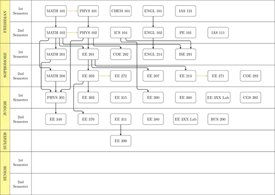
Placing Nodes

The nodes are getting placed via the online grid placement of the graphs library. This needs manual adjustments of distances between nodes (via x and y keys) since they're are just placed at the integer step of the x and y axis.

The node name * is used to skip a placement in the grid. The value \cols needs to be set inside the TikZ picture. It will be used to set up the grid placement as well as draw the lanes.

Multiple nodes of the same name, say *, will be named *, *', *'', etc. Besides the * “nodes” (which are meant to be used more than once), your diagram actually has a few nodes more than once. Since I didn't recreate the full diagram, in the code below, this only applies to the extra-wide EE 3XX Lab node.

---

A matrix would be much better but it will be no easy task to be also able to refer to those nodes by their content's name. A graph both sets the name and the content to the same value (if nothing else is specified).

Lanes

These are drawn around the grid's rows.

The loop are setup in a way that it allows the following list:

FRESHMAN/{1st, 2nd}, SOPHOMORE/{1st, 2nd},
JUNIOR/{1st, 2nd},   SUMMER/.,             SENIOR/{1st, 2nd}

The . (from SUMMER) means that no actual “Semester” label will be typeset (see key disable when .).

Node Setup (Graph 1)

Every node on the grid will get six extra anchors courtesy of add anchor to node, three at the top (in 1, in 2, in 3) and three at the bottom (out). This happens because all nodes in the first graph have outs = 3, ins = 3 as an option.

Since we can't create these anchors (which are coordinates turned anchors) directly while we're setting up the grid, we use a label which has special consideration by the graphs library.

This is also the reason we need two graphs.

If more out or in anchors are needed, they can be specified in the options of a node: MATH 102[outs=5].

Connecting Nodes (Graph 2)

A second graph with use existing nodes (i.e. those from the previous step) can now connect those nodes.

Here we use three kinds of connections:

1. A straight line that will be connect as they always woud.
2. A |-| connection from the ext.paths.ortho library. We can specify the anchors on both ends with oi = <out number>:<in number>.
3. An elbow connection that uses the following values and keys:

• out: the out anchor (this defaults to the middle one, 2, since all nodes are by default set up with three of those anchors),

• in: the in` anchor (same as above),

• oi = <out number>:<in number>, sets the previous two,

• | specified the vertical lane of the elbow connection, these 0 for the space between the first and second column and so forth, the value -1 stands for the vertical lane left of the first column.

  This key is not used in the code below because the elbow key is setup in a way that you can directly type that value of the vertical lane in the option of the elbow connection, i.e. elbow = {2, oi = 1:2} is the same as elbow = {| = 2, oi = 1:2}

• ok and ik specify the ratio for the first kink after the start node (out kink), the second for the ratio of the last kink before the target node.

  These ratios are set up so that 0 would put the kink at the border of the nodes while 1 would put it directly at the horizontal line of the Semester lanes.

• via and via distance specify a horizontal offset for the vertical connection.

  With the default values of via distance = 0.05, the following are the same:

  | = 2, via = 1
  | = 2.05
  

  because 2 + 1 × 0.05 = 2.05

It should be noted that these values can be set at the start of graph scope, i.e.

{[/tikz/elbow/|=3] c1 -> [elbow] c2, c3 -> [elbow] c4 }

and both those connection will use the values that are already set.

---

In a previous version, instead of having fixed anchors out 1, out 2 and so one, the starting point could be specified as a ratio as well (i.e. 0.5 would be the middle of the south or the north edge).

I don't know which one is better.

You can always set outs = 11, ins = 11 which would place eleven anchors at ¹/₁₂, ²/₁₂, …, ¹¹/₁₂ where out 2 would be the same as out 1 when outs = 5 would have been set or out 3 would be the same as out 1 under outs = 3.

Code

\documentclass[tikz]{standalone}
\usetikzlibrary{arrows.meta, calc, graphs, ext.paths.ortho}
\makeatletter
\def\@firstofgobble@until@relax#1#2\relax{#1}
\newcommand*\iftikznamestartswithstar{\if*\expandafter\@firstofgobble@until@relax\tikzgraphnodename\relax}
\tikzset{% https://tex.stackexchange.com/a/676090/16595
  add anchor to node/.code n args={3}{%
    \edef\tikz@temp##1{% \tikz@pp@name/\tikzlastnode needs to be expanded
      \noexpand\pgfutil@g@addto@macro\expandafter\noexpand\csname pgf@sh@ma@\tikz@pp@name{#1}\endcsname{%
        \def\expandafter\noexpand\csname pgf@anchor@\csname pgf@sh@ns@\tikz@pp@name{#1}\endcsname @#2\endcsname{##1}}}%
    \tikz@temp{#3}},
  add anchor to node*/.code n args={3}{% 1: node, 2: anchor, 3: coordinate
    \begingroup
      \pgfsettransform{\csname pgf@sh@nt@\tikz@pp@name{#1}\endcsname}%
      \pgf@process{\pgfpointanchor{\tikz@pp@name{#3}}{center}}%
      \pgfkeysalso{/tikz/add anchor to node/.expanded={#1}{#2}{\noexpand\pgfqpoint{\the\pgf@x}{\the\pgf@y}}}%
    \endgroup}}
\pgfqkeys{/pgf/foreach}{% https://tex.stackexchange.com/a/110823/16595
  global remember/.code=\pgfutil@append@tomacro{\pgffor@remember@code}{\gdef\noexpand#1{#1}}}
\newcommand*\tikzelbowset{\pgfqkeys{/tikz/elbow}}
\tikzelbowset{
  label/.style n args={4}{
    shape=coordinate,name=elbow@temp,anchor=center,tikz@label@post/.code 2 args=,
    at={($(\tikzlastnode.#2 west)!elbowAbs(#3,#4)!(\tikzlastnode.#2 east)$)},
    append after command/.expanded={[add anchor to node*={\tikzlastnode}{#1 #3}{elbow@temp}]}},
  via distance/.initial=.05,
  out/.initial=2, in/.initial=2, oi/.style args={#1:#2}{/tikz/elbow/out={#1},/tikz/elbow/in={#2}},
  ok/.initial=.5, ik/.initial=.5, via/.initial=0,
  |/.initial=0, .unknown/.code=\pgfkeyssetevalue{/tikz/elbow/|}{\pgfkeyscurrentname},
  .style={to path={\pgfextra{\tikzelbowset{#1}}
    coordinate (elbow@out)      at (\tikztostart .out \pgfkeysvalueof{/tikz/elbow/out})
    coordinate (elbow@in)       at (\tikztotarget.in  \pgfkeysvalueof{/tikz/elbow/in})
    coordinate (elbow@out kink) at (elbow@out|-{$(\tikztostart.south)!\pgfkeysvalueof{/tikz/elbow/ok}!([shift=(up:.5)]\tikztostart.center)$})
    coordinate (elbow@in  kink) at (elbow@in|-{$(\tikztotarget.north)!1-\pgfkeysvalueof{/tikz/elbow/ik}!([shift=(down:.5)]\tikztotarget.center)$})
    coordinate (elbow@)         at ({\pgfkeysvalueof{/tikz/elbow/|}+.5+\pgfkeysvalueof{/tikz/elbow/via distance}*\pgfkeysvalueof{/tikz/elbow/via}},0)
    (elbow@out) -- (elbow@out kink) -- (elbow@|-elbow@out kink) -- (elbow@|-elbow@in kink) \tikztonodes -- (elbow@in kink) -- (elbow@in)}}}
\tikzset{
  elbows/.code=\tikzelbowset{#1},
  outs/.style={/tikz/elbow/temp/.style={label={[/tikz/elbow/label={out}{south}{##1}{#1}]}},/tikz/elbow/temp/.list={1,...,#1}},
  ins/.style ={/tikz/elbow/temp/.style={label={[/tikz/elbow/label={in} {north}{##1}{#1}]}},/tikz/elbow/temp/.list={1,...,#1}}}
\pgfset{declare function={elbowRel(\i,\n)=(\i-(\n-1)/2); elbowAbs(\i,\n)=\i/(\n+1);}}
\begin{document}
\begin{tikzpicture}[
  x=3cm, y=-2cm,
  disable when ./.style={coordinate},
  gen/.style={fill=yellow!50},
  gen width/.initial=.9cm,
  sem width/.initial=2cm,
  subj/.style={draw, rounded corners, minimum width=1.9cm, minimum height=1cm},
]
\newcommand*\cols{7}
\foreach[count=\row from 0, remember=\row as \lastRow (initially -1)] \GEN/\SEM in {
  FRESHMAN/{1st, 2nd}, SOPHOMORE/{1st, 2nd}, JUNIOR/{1st, 2nd}, SUMMER/., SENIOR/{1st, 2nd}}{
  \let\firstRow\row \let\row\lastRow
  \foreach[remember=\row as \lastRow (initially \row), global remember=\lastRow] \SEMESTER in \SEM {
    \pgfmathtruncatemacro\row{\lastRow+1}
    \draw[shift=(up:\row)] (-.75,-.5) coordinate (@) rectangle ++(\cols+.5,1)
      (@) rectangle node[disable when \SEMESTER/.try, align=center]{\SEMESTER\\Semester}
      ++(-\pgfkeysvalueof{/tikz/sem width},1) coordinate (@);}
  \draw[gen] (@) rectangle node[rotate=90]{\GEN} ([xshift=-\pgfkeysvalueof{/tikz/gen width}]0,\firstRow-.5-|@);
  \let\row\lastRow}
\graph[
  grid placement, wrap after=\cols, branch up, % because y is inverted
  nodes={subj, \iftikznamestartswithstar coordinate\fi, outs=3, ins=3},
  fresh nodes,
]{% * = empty place in the grid
    MATH 101,         PHYS 101,         CHEM 101, ENGL 101, IAS 121,     *,           *,
    MATH 102[outs=5], PHYS 102,         ICS  104, ENGL 102, PE  101,     IAS 111,     *,
    MATH 201,         EE   201[outs=5], COE  202, ENGL 214, ISE 291,     *,           *,
    MATH 208,         EE   203,         EE   272, EE   207, EE  213,     EE  271,     COE 292,
    PHYS 305,         EE   303,         EE   315, EE   390, EE  360,     EE  3XX Lab, CGS 392,
    EE   340,         EE   370,         EE   311, EE   380, EE  3XX Lab, BUS 200,     *,
    *,                *,                EE   399,
};% one graph ends here because all the labels that create anchors need to be processed
\path[>={Triangle[scale=.75]}, thick, ortho/install shortcuts, rounded corners] graph[
  use existing nodes,
  oi/.style args={#1:#2}{left anchor=out #1,right anchor=in #2},
  or/.style={/tikz/ortho/ratio={#1}}]{
  {[edges=yellow!80!black] MATH 101 -> PHYS 101, MATH 102 -> PHYS 102, EE 203 -> EE 272, EE 213 -> EE 271},
  {
    MATH 101 -> MATH 102 -> MATH 201,
    PHYS 101 -> PHYS 102 -> EE   201,
    ENGL 101 -> ENGL 102 -> ENGL 214,
%    EE   201 ->[oi=1:2,|-|] EE   203,
    EE   201 ->             EE   203,
    MATH 208 ->             PHYS 305 -> EE 340,
    EE   203 ->             EE   303,
    EE   311 ->             EE   399,
  },
  MATH 102 ->[elbow={-1, oi=1:1}]        MATH 208,
  MATH 201 ->[elbow={-1, via=1, oi=1:1}] PHYS 305,
  MATH 102 ->[oi=4:1, |-|, or=.75]       EE   201,
  MATH 102 ->[oi=5:1, |-|, or=.6]        ISE  291,
  PHYS 102 ->[elbow={0, via=-1, oi=1:3}] PHYS 305,
  EE   203 ->[elbow={0, via=1,  oi=1:1}] EE   370,
  PHYS 102 ->[oi=3:2, |-|, or=.75]       COE  202,
  EE   201 ->[oi=4:1, |-|, or=.75]       EE   207,
  EE   201 ->[oi=5:2, |-|, or=.6]        EE   213,
  ICS  104 ->[oi=3:3, |-|, or=.25]       ISE  291,
  ICS  104 ->[elbow={2, ok=.75, oi=2:1}] EE   390,
};
\end{tikzpicture}
\end{document}

Output