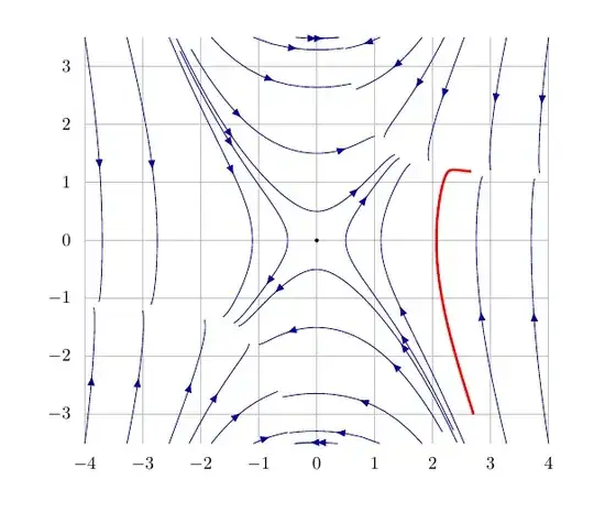
I tried to obtain a "stream plot" using basic TikZ. Each trajectory (or orbit) is constructed starting from a point and going forward and respectively backward in time. Considering your specific problem, my code does not cover the case of closed orbits. A different branch must be added inside the command \streamPlot.
The above drawing uses to sets of orbits constructed with stream plot by name and stream plot TB (top bottom). Note that these are pic objects so they should be handled with care in case scaling is used globally. They are based on \streamPlot.
I needed both since I consider that one needs to go closer to the singular points of the vector field to have a good image. For example, the image constructed with Mathematica doesn't really show what is happening near the origin.
Some remarks about the vector field that is considered: some rewriting is in order to arrive at a form that might be used with TikZ (a low computation accuracy, but enough for drawing). Below is one way of looking at the two components. I added a Taylor polynomial in x needed to understand the behavior for small values of x.
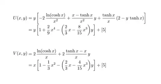
Remarks
Looking at the stream plot in the first drawing, it can be noticed that something is happening where trajectories "meet". To understand the issue, we can draw the vector field together with the curves U(x, y)=0 (in blue) and V(x, y)=0 (in red).
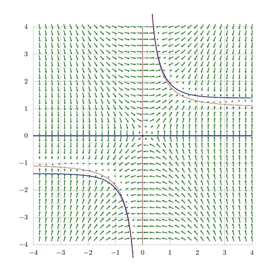 See also the last image below build with Python (this is why it is at the end of my answer).
The singularities of the vector field do not follow the blue curve (let's say) completely. But we cannot see this in the stream plot (Fig. 1). This is why I added the solution of the corresponding differential equation in red for a certain initial condition. It uses the function ode-trajectory.
The algorithm behind all the computations is the classical Runge-Kutta developed in the style runge-kutta.
The code
The code is rather long mainly because the vector field components are defined three times each (needed for different contexts), and because the graphical elements are of three types: vector field, stream plot, trajectory of a Cauchy problem.
\documentclass[11pt, margin=17pt]{standalone}
\usepackage{amsmath, amssymb}
\usepackage{ifthen}
\usepackage{tikz}
\usetikzlibrary{math, calc, arrows.meta}
\usetikzlibrary{decorations.markings}
\pgfkeys{/tikz/.cd,
  x bound start/.store in=\xBoundStart,
  x bound end/.store in=\xBoundEnd,
  y bound start/.store in=\yBoundStart,
  y bound end/.store in=\yBoundEnd
}
\makeatletter
\tikzset{%
  bounds/.style n args={4}{%
    evaluate={%
      \xBoundStart = #1;
      \xBoundEnd = #2;
      \yBoundStart = #3;
      \yBoundEnd = #4;
    }
  },
  pics/vector field background/.style={% axes + grid for a vector field
    code={%
      \begin{scope}[every node/.style={scale=.8},
        evaluate={%
          \iIni = {int(\xBoundStart)};
          \iEnd = {int(\xBoundEnd)};
          \jIni = {int(\yBoundStart)};
          \jEnd = {int(\yBoundEnd)};
        }]
        \draw[gray!50] (\xBoundStart, \yBoundStart)
        grid (\xBoundEnd, \yBoundEnd);
        \fill[black] (0, 0) circle (1pt);
        \foreach \i in {\iIni, ..., \iEnd}{%
          \path (\i, \yBoundStart) node[below=1ex] {$\i$};
        }
        \foreach \j in {\jIni, ..., \jEnd}{%
          \path (\xBoundStart, \j) node[left=1ex] {$\j$};
        }

      \end{scope}
    }
  },
  flow/.style={%  create a directional arrow along a trajectory
    decoration={
      markings,% switch on markings
      mark=at position .5 with {\arrow[#1]{Latex}}
    }, postaction=decorate
  },
  -flow/.style={%
    decoration={
      markings,% switch on markings
      mark=at position .5 with {\arrowreversed[#1]{Latex}}
    }, postaction=decorate
  },
  runge-kutta/.style={%  to be invoked before using ode-trajectory, ...
    evaluate={%
      int \N@ode, \i, \j;
      \N@ode = 4;
      for \i in {1, ..., \N@ode}{%
        for \j in {1, ..., \N@ode}{%
          \a@ode{\i,\j} = 0;
        };
      };
      \a@ode{2,1} = 1/2; \a@ode{3,2} = 1/2; \a@ode{4,3} = 1;
      \c@ode{1} = 0; \c@ode{2} = 1/2; \c@ode{3} = 1/2; \c@ode{4} = 1;
      \b@ode{1} = 1/6; \b@ode{2} = 1/3; \b@ode{3} = 1/3; \b@ode{4} = 1/6;
    }
  },
  % for ode in two dimensions
  ode-trajectory/.style args={RHTx=#1, RHTy=#2, from=#3, to=#4, steps=#5}{%
    insert path={coordinate (tmp) let \p1 = (tmp) in},
    evaluate={%
      real \showpointr, \testTmp;
      \showpointr = 1;
      int \steps@ode, \i, \j, \k, \s;
      \t@ode{0} = #3;
      \u@ode{0} = \x10.0352778;  % converts pt to cm
      \v@ode{0} = \y10.0352778;
      \steps@ode = int(#5);
      \t@ode{\steps@ode} = #4;
      \h = (\t@ode{\steps@ode} -\t@ode{0})/\steps@ode;
      for \s in {1, 2, ..., \steps@ode}{
        \k = int(\s -1);
        \t@ode{0,1} = \t@ode{\k};
        \x@ode{0,1} = \u@ode{\k};
        \y@ode{0,1} = \v@ode{\k};
        \qx@ode{0,1} = #1(\t@ode{0,1}, \x@ode{0,1}, \y@ode{0,1});
        \qy@ode{0,1} = #2(\t@ode{0,1}, \x@ode{0,1}, \y@ode{0,1});
        for \i in {2, ..., \N@ode}{%
          \t@ode{0,\i} = \t@ode{\k} +\h\c@ode{\i};
          \x@ode{0,\i} = \u@ode{\k};
          \y@ode{0,\i} = \v@ode{\k};
          for \j in {1, ..., {int(\i -1)}}{%
            \x@ode{0,\i} = \x@ode{0,\i} +\h\a@ode{\i,\j}\qx@ode{0,\j};
            \y@ode{0,\i} = \y@ode{0,\i} +\h\a@ode{\i,\j}\qy@ode{0,\j};
          };
          \qx@ode{0,\i} = #1(\t@ode{0,\i}, \x@ode{0,\i}, \y@ode{0,\i});
          \qy@ode{0,\i} = #2(\t@ode{0,\i}, \x@ode{0,\i}, \y@ode{0,\i});
        };
        \t@ode{\s} = \t@ode{\k} +\h;
        \u@ode{\s} = \u@ode{\k};
        \v@ode{\s} = \v@ode{\k};
        for \i in {1, 2, ..., \N@ode}{%
          \u@ode{\s} = \u@ode{\s} +\h\b@ode{\i}\qx@ode{0,\i};
          \v@ode{\s} = \v@ode{\s} +\h\b@ode{\i}\qy@ode{0,\i};
        };
      };
      \k = \steps@ode-1;
      \testTmp = pow(pow(\u@ode{\steps@ode} -\u@ode{\k}, 2)
      +pow(\v@ode{\steps@ode} -\v@ode{\k}, 2), .5);
    },
    insert path={%
      \foreach \s in {1, ..., \steps@ode}{
        -- (\u@ode{\s}, \v@ode{\s})
      }
    }
  },
  m vector field/.style n args={5}{% u / v / Nx / Ny / arrow scale
    insert path = {%
      \pgfextra{%
        \let\tikz@mode@save=\tikz@mode
        \let\tikz@options@save=\tikz@options%
      }
    },
    evaluate={%
      coordinate \tmp@P, \tmp@V;
      integer \Nx, \Ny;
      \Nx = #3;
      \Ny = #4;
      real \dx, \dy, \tmp, \uVF, \vVF, \nVF, \s@cst;
      \s@cst = .49;
      \dx = (\xBoundEnd -\xBoundStart)/\Nx;
      \dy = (\yBoundEnd -\yBoundStart)/\Ny;
      for \i in {1, ..., \Nx}{%
        for \j in {1, ..., \Ny}{%
          \uVF = #1(\xBoundStart -\dx/2 +\i\dx, \yBoundStart -\dy/2 +\j\dy);
          \vVF = #2(\xBoundStart -\dx/2 +\i\dx, \yBoundStart -\dy/2 +\j\dy);
          \nVF = pow(\uVF\uVF +\vVF\vVF, .5);
          if  \nVF > \s@cst then {%
            \uVF = \uVF/\nVF.5;
            \vVF = \vVF/\nVF.5;
          };
          \tmp@P = (\xBoundStart +\i\dx, \yBoundStart +\j\dy);
          \tmp@V = (#5\uVF, #5\vVF);
          {
            \draw[arrows={-Latex[width=2.5pt, length=2pt]}]
            \pgfextra{\let\tikz@mode=\tikz@mode@save
              \let\tikz@options=\tikz@options@save}
            ($(\tmp@P) -.5(\tmp@V)$) -- ++(\tmp@V);
          };

        };
      };
    }
  }
}
\newcommand{\streamPlot}[7]{% RHTx, RHTy, h, px, py, min, color
  \tikzmath{%
    integer \steps@ode, \i, \j, \k, \s, flag;
    real \h, \nor;
    \flag = 0;
    \s = 0;
    \k = 0;
    \h = #3;

    \u@ode{0} = #4;
    \v@ode{0} = #5;
    \t@ode{0} = 0;
  },
  \whiledo{\equal{\flag}{0}}{%
    \tikzmath{
      \s = \s +1;
      \t@ode{0,1} = 0;
      \x@ode{0,1} = \u@ode{\k};
      \y@ode{0,1} = \v@ode{\k};
      \qx@ode{0,1} = #1(\t@ode{0,1}, \x@ode{0,1}, \y@ode{0,1});
      \qy@ode{0,1} = #2(\t@ode{0,1}, \x@ode{0,1}, \y@ode{0,1});
      for \i in {2, ..., \N@ode}{%
        \t@ode{0,\i} = \t@ode{\k} +\h\c@ode{\i};
        \x@ode{0,\i} = \u@ode{\k};
        \y@ode{0,\i} = \v@ode{\k};
        for \j in {1, ..., {int(\i -1)}}{%
          \x@ode{0,\i} = \x@ode{0,\i} +\h\a@ode{\i,\j}\qx@ode{0,\j};
          \y@ode{0,\i} = \y@ode{0,\i} +\h\a@ode{\i,\j}\qy@ode{0,\j};
        };
        \qx@ode{0,\i} = #1(\t@ode{0,\i}, \x@ode{0,\i}, \y@ode{0,\i});
        \qy@ode{0,\i} = #2(\t@ode{0,\i}, \x@ode{0,\i}, \y@ode{0,\i});
      };
      \t@ode{\s} = \t@ode{\k} +\h;
      \u@ode{\s} = \u@ode{\k};
      \v@ode{\s} = \v@ode{\k};
      for \i in {1, 2, ..., \N@ode}{%
        \u@ode{\s} = \u@ode{\s} +\h\b@ode{\i}\qx@ode{0,\i};
        \v@ode{\s} = \v@ode{\s} +\h\b@ode{\i}*\qy@ode{0,\i};
      };
      \nor = pow(%
        pow(\u@ode{\s} -\u@ode{\k}, 2) +pow(\v@ode{\s} -\v@ode{\k}, 2),
      .5);
      if \nor<#6 then {\flag = 1;};
      if \u@ode{\s}<\xBoundStart then {\flag = 1;};
      if \u@ode{\s}>\xBoundEnd then {\flag = 1;};
      if \v@ode{\s}<\yBoundStart then {\flag = 1;};
      if \v@ode{\s}>\yBoundEnd then {\flag = 1;};
      \k = \k +1;
    }
  },
  \tikzmath{%
    if \s>1 then {%
      if #3>0 then {%
        {%
          \draw[#7, flow={#7}]  (\u@ode{0}, \v@ode{0})
          \foreach \i [parse=true] in {1, ..., \s-1}{
            -- (\u@ode{\i}, \v@ode{\i})
          };
        };
      } else {%
        {%
          \draw[#7, -flow={#7}]  (\u@ode{0}, \v@ode{0})
          \foreach \i [parse=true] in {1, ..., \s-1}{
            -- (\u@ode{\i}, \v@ode{\i})
          };
        };
      };
    };
  }
}
\makeatother
\tikzset{
  pics/stream plot by name/.style args={RHTx=#1, RHTy=#2, dT=#3, pName=#4,
    pNumber=#5, min=#6, color=#7}{%
    code={
      \foreach \i in {1, ..., #5}{%
        \tikzmath{%
          coordinate \P;
          \P = (#4-\i);
          \px = \Px1pt/1cm;  % converts pt to cm
          \py = \Py1pt/1cm;
        }
        % \draw (\px, \py) circle (2pt);
        \streamPlot{#1}{#2}{#3}{\px}{\py}{#6}{#7};
        \streamPlot{#1}{#2}{-#3}{\px}{\py}{#6}{#7};
      }
    }
  },
  pics/stream plot TB/.style args={%
    RHTx=#1, RHTy=#2, dT=#3, uSteps=#4, min=#5, color=#6}{%
    code={
      \tikzmath{%
        real \px, \py, \dx;
        \dx = (\xBoundEnd -\xBoundStart)/#4;
      }
      \foreach \i in {0, ..., #4}{%
        \tikzmath{%
          \px = \xBoundStart +\i\dx;
          \py = \yBoundStart;
        }
        \streamPlot{#1}{#2}{#3}{\px}{\py}{#5}{#6};
        \streamPlot{#1}{#2}{-#3}{\px}{\py}{#5}{#6};
      }
      \foreach \i in {0, ..., #4}{%
        \tikzmath{%
          \px = \xBoundStart +\i\dx;
          \py = \yBoundEnd;
        }
        \streamPlot{#1}{#2}{#3}{\px}{\py}{#5}{#6};
        \streamPlot{#1}{#2}{-#3}{\px}{\py}{#5}{#6};
      }
    }
  }
}
\begin{document}
%\iffalse
\begin{tikzpicture}[every node/.style={%
    right, align=left, inner sep=3ex
  }]
  \path (-1.3, 0) node {$U(x, y)$}
  (0, 0) node[] {$\displaystyle
    = y\left[
      -2,\frac{\ln(\cosh x)}{x^2}
      +\frac{x -\tanh x}{x^2},y
      +\frac{\tanh x}{x},(2 -y,\tanh x)
    \right]$}
  ++(0, -1) node[] {$\displaystyle
    = y\left[
      1 +\frac{2}{9},x^4
      -\bigg(\frac{2}{3},x -\frac{8}{15},x^3\bigg)y
    \right] +[5]$};
\path (-1.3, -3) node {$V(x, y)$}
  (0, -3) node[] {$\displaystyle
    = 2,\frac{\ln(\cosh x)}{x} +2,\frac{\tanh x -x}{x},y$}
  ++(0, -1) node[] {$\displaystyle
    = x\left[
      1 -\frac{1}{3},x^2
      -\bigg( \frac{2}{3},x -\frac{4}{15},x^3 \bigg)y
    \right] +[5]$};
\end{tikzpicture}
%\fi
\tikzmath{%
  function Ux(\t, \u, \v) {%
    real \a, \b, \c;
    if abs(\u)>.05 then {%
      \a = -2ln(cosh(\u))/(\u\u);
      \b = (\u -tanh(\u))/(\u\u)\v;
      \c = (tanh(\u)/\u)(2 - tanh(\u)\v);
    } else {%
      \a = 1 -2/3\u\v;
      \b = 8/15pow(\u, 3)\v;
      \c = 2/9pow(\u, 4);
    };
    return {(\a +\b +\c)\v};
  };
  function Uy(\t, \u, \v) {%
    real \a, \b;
    if abs(\u)>.05 then {%
      \a = ln(cosh(\u))/\u;
      \b = (tanh(\u) -\u)/\u;
      return {2\a +2\b\v};
    } else {
      \a = 1 -pow(\u, 2)/3;
      \b = -(2/3)\u +(4/15)pow(\u, 3);
      return {\u(\a +\b\v)};
    };
  };
  function fUy(\u) {%
    real \a, \b;
    \a = ln(cosh(\u))/\u;
    \b = (\u -tanh(\u))/\u;
    return \a/\b;
  };
  function UxVF(\u, \v) {%
    real \a, \b, \c;
    if abs(\u)>.05 then {%
      \a = -2ln(cosh(\u))/(\u\u);
      \b = (\u -tanh(\u))/(\u\u)\v;
      \c = (tanh(\u)/\u)(2 - tanh(\u)\v);
    } else {%
      \a = 1 -2/3\u\v;
      \b = 8/15pow(\u, 3)\v;
      \c = 2/9pow(\u, 4);
    };
    return {(\a +\b +\c)\v};
  };
  function fUx(\u) {%
    real \a, \b;
    \a = 2(tanh(\u)/\u) -2ln(cosh(\u))/(\u\u);
    \b = -(\u -tanh(\u))/(\u\u) +(tanh(\u)/\u)tanh(\u);
    return \a/\b;
  };
  function UyVF(\u, \v) {%
    real \a, \b;
    if abs(\u)>.05 then {%
      \a = ln(cosh(\u))/\u;
      \b = (tanh(\u) -\u)/\u;
      return {2\a +2\b\v};
    } else {
      \a = 1 -pow(\u, 2)/3;
      \b = -(2/3)\u +(4/15)pow(\u, 3);
      return {\u(\a +\b*\v)};
    };
  };
}
\iffalse
\begin{tikzpicture}
  \draw[gray!50, very thin] (-3.5, -3.25) grid (3.5, 3.25);
  \draw[->] (-3.5, 0) -- (3.5, 0) node[above right] {$x$};
  \draw[->] (0,-3.5) -- (0, 3.5) node[left] {$y$};
\draw[blue!70!black, thick, variable=\t, domain=.5:3.25, samples=200]
  plot (\t, {fUx(\t)});
  \draw[blue!70!black, thick] (-3.25, 0) -- (3.25, 0);
  \draw[blue!70!black, thick, variable=\t, domain=-3.25:-.5, samples=200]
  plot (\t, {fUx(\t)});
  \draw[red, thin, variable=\t, domain=.5:3.25, samples=200]
  plot (\t, {fUy(\t)});
  \draw[red] (-0, -3.25) -- (0, 3.25);
  \draw[red, thin, variable=\t, domain=-3.25:-.5, samples=200]
  plot (\t, {fUy(\t)});
\end{tikzpicture}
\fi
\iffalse
\begin{tikzpicture}[runge-kutta, bounds={-4}{4}{-4}{4}, scale=1.2]
  \path pic[scale=1.2] {vector field background};
\draw[blue!70!black, thick,
  variable=\t, domain=.35:\xBoundEnd, samples=200]
  plot (\t, {fUx(\t)});
  \draw[blue!70!black, thick] (\xBoundStart, 0) -- (\xBoundEnd, 0);
  \draw[blue!70!black, thick,
  variable=\t, domain=\xBoundStart:-.35, samples=200]
  plot (\t, {fUx(\t)});
  \draw[red, thin, variable=\t, domain=.35:\xBoundEnd, samples=200]
  plot (\t, {fUy(\t)});
  \draw[red] (-0, \xBoundStart) -- (0, \xBoundEnd);
  \draw[red, thin, variable=\t, domain=\xBoundStart:-.35, samples=200]
  plot (\t, {fUy(\t)});
  \draw[green!50!black, thick, m vector field={UxVF}{UyVF}{35}{35}{.4}];
\end{tikzpicture}
\fi
\iffalse
\begin{tikzpicture}[runge-kutta, bounds={-4}{4}{-3.5}{3.5}]
  \path pic {vector field background};
% A points
  \path (0, 1.5) coordinate (A-1);
  \path (0, -1.5) coordinate (A-2);
  \path (2.2, \yBoundEnd) coordinate (A-3);
  \path (-2.2, \yBoundStart) coordinate (A-4);
% B points
  \tikzmath{
    integer \N;
    \N = 4;
  }
  \foreach \i in {1, ..., \N}{%
    \path (\i*360/\N: .5) coordinate (B-\i);
  }
\path pic {stream plot by name={RHTx=Ux, RHTy=Uy, dT=.05,
      pName=A, pNumber=4, min=.005, color=blue!60!black}};
  \path pic {stream plot by name={RHTx=Ux, RHTy=Uy, dT=.05,
      pName=B, pNumber=\N, min=.005, color=blue!60!black}};
\path pic {stream plot TB={RHTx=Ux, RHTy=Uy, dT=.05,
      uSteps=11, min=.005, color=blue!60!black}};
\draw[red, very thick] (2.7, -3)
  [ode-trajectory={RHTx=Ux, RHTy=Uy, from=0, to=15, steps=1500}];

\end{tikzpicture}
\fi
\end{document}
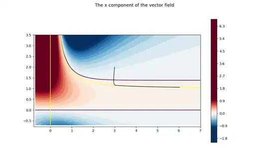
The level curves of the U component of the vector field. The red curve from Fig. 1 is the black trajectory here!