1

My MWE:

\documentclass{scrreprt}
\usepackage{tikz}

\usetikzlibrary{datavisualization.formats.functions} \pgfooclass{circle visualizer}{%from TikZ & PGF manual, page 928 \attribute name; \method circle visualizer(#1) {\pgfooset{name}{#1}} \method default connects() { \pgfoothis.get handle(\me) \pgfkeysvalueof{/pgf/data visualization/obj}.connect(\me,visualize,visualize datapoint signal) } \method visualize() { \pgfdvfilterpassedtrue \pgfdvnamedvisualizerfilter \ifpgfdvfilterpassed \dovisualization \fi } } \def\dovisualization{ \pgfkeysvalueof{/data point/\pgfoovalueof{name}/execute at begin} \pgfpathcircle{\pgfpointdvdatapoint}{\pgfkeysvalueof{/data point/radius}} \pgfkeysvalueof{/data point/\pgfoovalueof{name}/execute at end} } \tikzdatavisualizationset{ visualize as circle/.style = { new object = { when = after survey, store = /tikz/data visualization/visualizers/#1, class = circle visualizer, arg1 = #1 }, new visualizer = {#1}{color = visualizer color, every path/.style = { draw, fill }, }{}, /data point/set = #1 }, visualize as circle/.default = circle } \begin{document} \begin{figure} \centering %pic 1 \begin{tikzpicture} \datavisualization[ scientific axes = clean, all axes = grid, x axis = {unit length = 10em per .5 units}, y axis = {ticks = {node style = { align = right, text width = 7.5mm } }, label = $\varphi_{\textnormal M1}$ in Grad }, visualize as line, every visualizer/.style = very thin ] data { x, y 0, -90 .04, -90 .08, -90 .12, -90 .16, -90 .2, -90 .24, -90 .28, -90 .32, -90 .36, -90 .4, -90 .44, -90 .48, -90 .52, -90 .56, -90 .6, -90 .64, -90 .68, -90 .72, -90 .76, -90 .8, -90 .84, -90 .88, -90 .92, -90 .96, -90 1, 90 1.04, 90 1.08, 90 1.12, 90 1.16, 90 1.2, 90 1.24, 90 1.28, 90 1.32, -90 1.36, -90 1.4, -90 1.44, -90 1.48, -90 1.52, -90 1.56, -90 }; \end{tikzpicture}

%pic 2
\begin{tikzpicture}
  \datavisualization[
                     scientific axes = clean,
                     all axes = grid,
                     x axis = {unit length = 10em per .5 units},
                     y axis = {ticks = {node style = {
                                                      align = right,
                                                      text width = 7.5mm
                                                     }
                                       },
                               label = $\varphi_{\textnormal M2}$ in Grad
                              },
                     visualize as line,
                     every visualizer/.style = very thin
                    ]
  data {
        x,    y
        0,     90
         .04,  90
         .08,  90
         .12, -90
         .16, -90
         .2,  -90
         .24, -90
         .28, -90
         .32,  90
         .36,  90
         .4,   90
         .44,  90
         .48,  90
         .52, -90
         .56, -90
         .6,  -90
         .64, -90
         .68, -90
         .72, -90
         .76, -90
         .8,   90
         .84,  90
         .88,  90
         .92,  90
         .96,  90
        1,    -90
        1.04, -90
        1.08, -90
        1.12, -90
        1.16, -90
        1.2,  -90
        1.24, -90
        1.28, -90
        1.32, -90
        1.36, -90
        1.4,  -90
        1.44, -90
        1.48, -90
        1.52,  90
        1.56,  90
       };
\end{tikzpicture}

%pic 3
\begin{tikzpicture}
  \datavisualization[
                     scientific axes = clean,
                     all axes = grid,
                     x axis = {unit length = 10em per .5 units},
                     y axis = {ticks = {node style = {
                                                      align = right,
                                                      text width = 7.5mm
                                                     }
                                       },
                               label = $\varphi_1$ in Grad
                              },
                     visualize as circle
                    ]
  data {
        x,    y,      radius
        0,      0,    .25pt
         .04,   -.54, .25pt
         .08,   -.9,  .25pt
         .12,  -2.7,  .25pt
         .16,  -6.3,  .25pt
         .2,  -11.52, .25pt
         .24, -17.82, .25pt
         .28, -25.2,  .25pt
         .32, -33.3,  .25pt
         .36, -41.94, .25pt
         .4,  -50.58, .25pt
         .44, -58.86, .25pt
         .48, -66.78, .25pt
         .52, -73.98, .25pt
         .56, -80.28, .25pt
         .6,  -85.32, .25pt
         .64, -89.46, .25pt
         .68, -92.34, .25pt
         .72, -94.14, .25pt
         .76, -95.04, .25pt
         .8,  -95.04, .25pt
         .84, -94.5,  .25pt
         .88, -93.6,  .25pt
         .92, -92.52, .25pt
         .96, -91.44, .25pt
        1,    -90.72, .25pt
        1.04, -90.36, .25pt
        1.08, -89.82, .25pt
        1.12, -88.56, .25pt
        1.16, -85.14, .25pt
        1.2,  -79.02, .25pt
        1.24, -70.38, .25pt
        1.28, -59.76, .25pt
        1.32, -47.34, .25pt
        1.36, -33.84, .25pt
        1.4,  -19.98, .25pt
        1.44,  -7.2,  .25pt
        1.48,   2.52, .25pt
        1.52,   8.46, .25pt
        1.56,  10.26, .25pt
       };
\end{tikzpicture}

%pic 4
\begin{tikzpicture}
  \datavisualization[
                     scientific axes = clean,
                     all axes = grid,
                     x axis = {unit length = 10em per .5 units},
                     y axis = {ticks = {node style = {
                                                      align = right,
                                                      text width = 7.5mm
                                                     }
                                       },
                               label = $\varphi_2$ in Grad
                              },
                     visualize as circle
                    ]
  data {
        x,    y,       radius
        0,       0,    .25pt
         .04,    -.54, .25pt
         .08,    -.54, .25pt
         .12,    -.54, .25pt
         .16,    -.72, .25pt
         .2,     -.72, .25pt
         .24,    -.9,  .25pt
         .28,   -1.26, .25pt
         .32,   -1.8,  .25pt
         .36,   -2.88, .25pt
         .4,    -4.68, .25pt
         .44,   -7.2,  .25pt
         .48,  -10.8,  .25pt
         .52,  -15.48, .25pt
         .56,  -21.24, .25pt
         .6,   -27.72, .25pt
         .64,  -34.92, .25pt
         .68,  -42.3,  .25pt
         .72,  -49.86, .25pt
         .76,  -57.42, .25pt
         .8,   -64.8,  .25pt
         .84,  -71.82, .25pt
         .88,  -78.48, .25pt
         .92,  -84.6,  .25pt
         .96,  -90.36, .25pt
        1,     -95.76, .25pt
        1.04, -100.62, .25pt
        1.08, -104.76, .25pt
        1.12, -108.18, .25pt
        1.16, -110.7,  .25pt
        1.2,  -111.96, .25pt
        1.24, -111.96, .25pt
        1.28, -110.52, .25pt
        1.32, -107.82, .25pt
        1.36, -103.68, .25pt
        1.4,   -98.28, .25pt
        1.44,  -91.44, .25pt
        1.48,  -83.52, .25pt
        1.52,  -74.52, .25pt
        1.56,  -64.98, .25pt
       };
\end{tikzpicture}

%pic5
\begin{tikzpicture}
  \datavisualization[
                     scientific axes = clean,
                     all axes = grid,
                     x axis = {
                               unit length = 10em per .5 units,
                               label = $t$ in s
                              },
                     y axis = {label = $\varphi_3$ in Grad},
                     visualize as circle
                    ]
  data {
        x,    y,       radius
        0,       0,    .25pt
         .04,    -.36, .25pt
         .08,    -.36, .25pt
         .12,     .36, .25pt
         .16,    2.7,  .25pt
         .2,     5.94, .25pt
         .24,    7.92, .25pt
         .28,    7.56, .25pt
         .32,    5.04, .25pt
         .36,     .36, .25pt
         .4,    -5.22, .25pt
         .44,   -9.18, .25pt
         .48,  -10.98, .25pt
         .52,  -10.62, .25pt
         .56,   -8.28, .25pt
         .6,    -5.22, .25pt
         .64,   -3.96, .25pt
         .68,   -5.22, .25pt
         .72,   -9.18, .25pt
         .76,  -15.48, .25pt
         .8,   -23.94, .25pt
         .84,  -34.56, .25pt
         .88,  -46.8,  .25pt
         .92,  -59.58, .25pt
         .96,  -70.38, .25pt
        1,     -77.94, .25pt
        1.04,  -82.44, .25pt
        1.08,  -83.52, .25pt
        1.12,  -82.8,  .25pt
        1.16,  -82.26, .25pt
        1.2,   -82.62, .25pt
        1.24,  -83.88, .25pt
        1.28,  -85.86, .25pt
        1.32,  -88.56, .25pt
        1.36,  -91.8,  .25pt
        1.4,   -95.22, .25pt
        1.44,  -98.46, .25pt
        1.48, -101.52, .25pt
        1.52, -103.86, .25pt
        1.56, -105.3,  .25pt
       };
\end{tikzpicture}

\end{figure} \end{document}

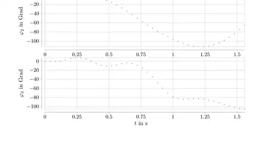
creates the following figure

result

Before you start: For every \begin{tikzpicture}...\end{tikzpicture} in this question I use in real \input{path/picNumber.tex} with the content \begin{tikzpicture}...\end{tikzpicture}. For this question I use only \begin{tikzpicture}...\end{tikzpicture} for a better understanding.

As you can see the label of the x-axis is shifted. Why? This only appears if I introduce a custom unit length between the ticks of the x axis, for example unit length = 10em per .5 units. I'm using a custom unit length between the ticks of the x axis to stretch the width of the figures, because in real I have thousands of data points and if I leave the standard unit length between the ticks of the x axis then my figures getting just black boxes, because ot the amount of data.

How can one center the shifted label?

Thank you for your help and effort in advance!
Su-47
  • 2,508

1 Answers1

1

The key label={[<options>]<text>} key sets the label of an axis to <text>. This text will be placed inside a node and the <options> can be used to configure the way this node is rendered. You must say node style to set the style of a node.

In this example, the node has been shifted to the right by 10em, which corresponds to 0.5 units, from 0.25 to 0.75.

a

\documentclass{scrreprt}
\usepackage{tikz}

\usetikzlibrary{datavisualization.formats.functions} \pgfooclass{circle visualizer}{%from TikZ & PGF manual, page 928 \attribute name; \method circle visualizer(#1) {\pgfooset{name}{#1}} \method default connects() { \pgfoothis.get handle(\me) \pgfkeysvalueof{/pgf/data visualization/obj}.connect(\me,visualize,visualize datapoint signal) } \method visualize() { \pgfdvfilterpassedtrue \pgfdvnamedvisualizerfilter \ifpgfdvfilterpassed \dovisualization \fi } } \def\dovisualization{ \pgfkeysvalueof{/data point/\pgfoovalueof{name}/execute at begin} \pgfpathcircle{\pgfpointdvdatapoint}{\pgfkeysvalueof{/data point/radius}} \pgfkeysvalueof{/data point/\pgfoovalueof{name}/execute at end} } \tikzdatavisualizationset{ visualize as circle/.style = { new object = { when = after survey, store = /tikz/data visualization/visualizers/#1, class = circle visualizer, arg1 = #1 }, new visualizer = {#1}{color = visualizer color, every path/.style = { draw, fill }, }{}, /data point/set = #1 }, visualize as circle/.default = circle } \begin{document} \begin{figure} \centering %pic 1 \begin{tikzpicture} \datavisualization[ scientific axes = clean, all axes = grid, x axis = {unit length = 10em per .5 units}, y axis = {ticks = {node style = { align = right, text width = 7.5mm } }, label = $\varphi_{\textnormal M1}$ in Grad }, visualize as line, every visualizer/.style = very thin ] data { x, y 0, -90 .04, -90 .08, -90 .12, -90 .16, -90 .2, -90 .24, -90 .28, -90 .32, -90 .36, -90 .4, -90 .44, -90 .48, -90 .52, -90 .56, -90 .6, -90 .64, -90 .68, -90 .72, -90 .76, -90 .8, -90 .84, -90 .88, -90 .92, -90 .96, -90 1, 90 1.04, 90 1.08, 90 1.12, 90 1.16, 90 1.2, 90 1.24, 90 1.28, 90 1.32, -90 1.36, -90 1.4, -90 1.44, -90 1.48, -90 1.52, -90 1.56, -90 }; \end{tikzpicture}

    %pic 2
    \begin{tikzpicture}
        \datavisualization[
        scientific axes = clean,
        all axes = grid,
        x axis = {unit length = 10em per .5 units},
        y axis = {ticks = {node style = {
                    align = right,
                    text width = 7.5mm
                }
            },
            label = $\varphi_{\textnormal M2}$ in Grad
        },
        visualize as line,
        every visualizer/.style = very thin
        ]
        data {
            x,    y
            0,     90
            .04,  90
            .08,  90
            .12, -90
            .16, -90
            .2,  -90
            .24, -90
            .28, -90
            .32,  90
            .36,  90
            .4,   90
            .44,  90
            .48,  90
            .52, -90
            .56, -90
            .6,  -90
            .64, -90
            .68, -90
            .72, -90
            .76, -90
            .8,   90
            .84,  90
            .88,  90
            .92,  90
            .96,  90
            1,    -90
            1.04, -90
            1.08, -90
            1.12, -90
            1.16, -90
            1.2,  -90
            1.24, -90
            1.28, -90
            1.32, -90
            1.36, -90
            1.4,  -90
            1.44, -90
            1.48, -90
            1.52,  90
            1.56,  90
        };
    \end{tikzpicture}

    %pic 3
    \begin{tikzpicture}
        \datavisualization[
        scientific axes = clean,
        all axes = grid,
        x axis = {unit length = 10em per .5 units},
        y axis = {ticks = {node style = {
                    align = right,
                    text width = 7.5mm
                }
            },
            label = $\varphi_1$ in Grad
        },
        visualize as circle
        ]
        data {
            x,    y,      radius
            0,      0,    .25pt
            .04,   -.54, .25pt
            .08,   -.9,  .25pt
            .12,  -2.7,  .25pt
            .16,  -6.3,  .25pt
            .2,  -11.52, .25pt
            .24, -17.82, .25pt
            .28, -25.2,  .25pt
            .32, -33.3,  .25pt
            .36, -41.94, .25pt
            .4,  -50.58, .25pt
            .44, -58.86, .25pt
            .48, -66.78, .25pt
            .52, -73.98, .25pt
            .56, -80.28, .25pt
            .6,  -85.32, .25pt
            .64, -89.46, .25pt
            .68, -92.34, .25pt
            .72, -94.14, .25pt
            .76, -95.04, .25pt
            .8,  -95.04, .25pt
            .84, -94.5,  .25pt
            .88, -93.6,  .25pt
            .92, -92.52, .25pt
            .96, -91.44, .25pt
            1,    -90.72, .25pt
            1.04, -90.36, .25pt
            1.08, -89.82, .25pt
            1.12, -88.56, .25pt
            1.16, -85.14, .25pt
            1.2,  -79.02, .25pt
            1.24, -70.38, .25pt
            1.28, -59.76, .25pt
            1.32, -47.34, .25pt
            1.36, -33.84, .25pt
            1.4,  -19.98, .25pt
            1.44,  -7.2,  .25pt
            1.48,   2.52, .25pt
            1.52,   8.46, .25pt
            1.56,  10.26, .25pt
        };
    \end{tikzpicture}

    %pic 4
    \begin{tikzpicture}
        \datavisualization[
        scientific axes = clean,
        all axes = grid,
        x axis = {unit length = 10em per .5 units},
        y axis = {ticks = {node style = {
                    align = right,
                    text width = 7.5mm
                }
            },
            label = $\varphi_2$ in Grad
        },
        visualize as circle
        ]
        data {
            x,    y,       radius
            0,       0,    .25pt
            .04,    -.54, .25pt
            .08,    -.54, .25pt
            .12,    -.54, .25pt
            .16,    -.72, .25pt
            .2,     -.72, .25pt
            .24,    -.9,  .25pt
            .28,   -1.26, .25pt
            .32,   -1.8,  .25pt
            .36,   -2.88, .25pt
            .4,    -4.68, .25pt
            .44,   -7.2,  .25pt
            .48,  -10.8,  .25pt
            .52,  -15.48, .25pt
            .56,  -21.24, .25pt
            .6,   -27.72, .25pt
            .64,  -34.92, .25pt
            .68,  -42.3,  .25pt
            .72,  -49.86, .25pt
            .76,  -57.42, .25pt
            .8,   -64.8,  .25pt
            .84,  -71.82, .25pt
            .88,  -78.48, .25pt
            .92,  -84.6,  .25pt
            .96,  -90.36, .25pt
            1,     -95.76, .25pt
            1.04, -100.62, .25pt
            1.08, -104.76, .25pt
            1.12, -108.18, .25pt
            1.16, -110.7,  .25pt
            1.2,  -111.96, .25pt
            1.24, -111.96, .25pt
            1.28, -110.52, .25pt
            1.32, -107.82, .25pt
            1.36, -103.68, .25pt
            1.4,   -98.28, .25pt
            1.44,  -91.44, .25pt
            1.48,  -83.52, .25pt
            1.52,  -74.52, .25pt
            1.56,  -64.98, .25pt
        };
    \end{tikzpicture}

    %pic5
    \begin{tikzpicture}
        \datavisualization[
        scientific axes = clean,
        all axes = grid,
        x axis = {
            unit length = 10em per .5 units,
            label={[node style={xshift= 10em}]{$t$ in s}},  %changed &lt;&lt;&lt;&lt;&lt;&lt;&lt;&lt;&lt;&lt;&lt;&lt;&lt;&lt;
        },
        y axis = {label = $\varphi_3$ in Grad},
        visualize as circle
        ]
        data {
            x,    y,       radius
            0,       0,    .25pt
            .04,    -.36, .25pt
            .08,    -.36, .25pt
            .12,     .36, .25pt
            .16,    2.7,  .25pt
            .2,     5.94, .25pt
            .24,    7.92, .25pt
            .28,    7.56, .25pt
            .32,    5.04, .25pt
            .36,     .36, .25pt
            .4,    -5.22, .25pt
            .44,   -9.18, .25pt
            .48,  -10.98, .25pt
            .52,  -10.62, .25pt
            .56,   -8.28, .25pt
            .6,    -5.22, .25pt
            .64,   -3.96, .25pt
            .68,   -5.22, .25pt
            .72,   -9.18, .25pt
            .76,  -15.48, .25pt
            .8,   -23.94, .25pt
            .84,  -34.56, .25pt
            .88,  -46.8,  .25pt
            .92,  -59.58, .25pt
            .96,  -70.38, .25pt
            1,     -77.94, .25pt
            1.04,  -82.44, .25pt
            1.08,  -83.52, .25pt
            1.12,  -82.8,  .25pt
            1.16,  -82.26, .25pt
            1.2,   -82.62, .25pt
            1.24,  -83.88, .25pt
            1.28,  -85.86, .25pt
            1.32,  -88.56, .25pt
            1.36,  -91.8,  .25pt
            1.4,   -95.22, .25pt
            1.44,  -98.46, .25pt
            1.48, -101.52, .25pt
            1.52, -103.86, .25pt
            1.56, -105.3,  .25pt
        };
    \end{tikzpicture}
\end{figure}

\end{document}

Simon Dispa
  • 39,141