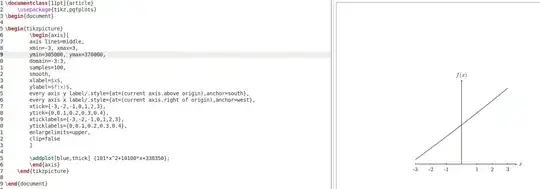
A little late but the short answer is to change your ymin and ymax: ymin=305000, ymax=380000,, adjust your y-axis labels as you see fit and change your function to 101*x^2+10100*x+338350. The result running in Gummi is:
That answer might seem a bit strange, so go to a Sage Cell Server and copy/paste the code below in
f=x^2
for i in range(1,101):
    f+=(x+i)^2
plot(f,-100,100)
then press Evaluate to get
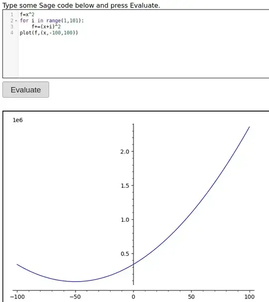
We're dealing with what looks like a parabola and if you think about it, each of the 101 terms in the sum is a quadratic. The x^2 terms all have coefficient 1, so the function has 101x^2. The x terms are 2x, 4x, ..., 200x so the coefficient of x is 2(1+2+...+100). There's a formula for that 2(100/2)(1+100). The constant terms are 1^2+2^2+3^2+...+100^2. There's a formula for that as well (1/6)(100)(100+1)(2(100)+1). The Sage cell server can do the work, though:
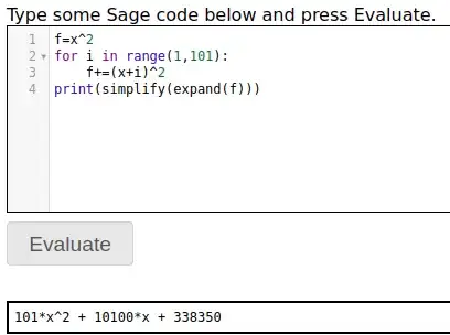
In a more general case, which couldn't be reasoned through, you can use the sagetex package, which relies on an open source computer algebra system to do the work. For this problem we could write
\documentclass{article}
\usepackage{sagetex,amsmath,amssymb,tikz,pgfplots}
\pgfplotsset{compat=1.18}
\begin{document}
\begin{sagesilent}
f=x^2
for i in range(1,101):
    f+=(x+i)^2
g=diff(f,x)
sol = solve(g==0,x)
\end{sagesilent}
Let $f(x,k)=\sum_{i=0}^{k}(x+i)^2$. For $k=100$ this becomes, after
explanding and collecting like terms, $f(x,100)=\sage{simplify(expand(f))}$
which is a parabola. Since $f'(x)=\sage{g}$ the minimum value is when
$x=\sage{sol[0].rhs()}$.
The plot of $f(x,100)$ looks like this over $[-3,3]$:
\begin{center}
\begin{tikzpicture}
\begin{axis}[axis lines=middle,xmin=-3,  xmax=3,ymin=305000,ymax=380000,domain=-3:3,samples=100,  smooth,xlabel=$x$,ylabel=$f(x)$, every axis y label/.style={at=(current axis.above origin), anchor=south},every axis x label/.style={at=(current axis.right of origin), anchor=west},xtick={-3,-2,-1,0,1,2,3},xticklabels={-3,-2,-1,0,1,2,3},enlargelimits=upper, clip=false]
\addplot[blue,thick] {101*x^2+10100*x+338350};
\end{axis}
\end{tikzpicture}
\end{center}
\end{document}
The result in Cocalc is:
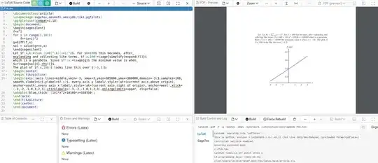
Note that f=x^2 for i in range(1,101):f+=(x+i)^2 defines the function (the last number, 101, doesn't get executed in Python). I can pull up the expansion \sage{simplify(expand(f))}, calculate its derivative, g=diff(f,x) and find the value of the minimum sol = solve(g==0,x). These values can then be put into the LaTeX document.
Sage is not part of LaTeX so you will need a free Cocalc account or download Sage to your computer.


