1

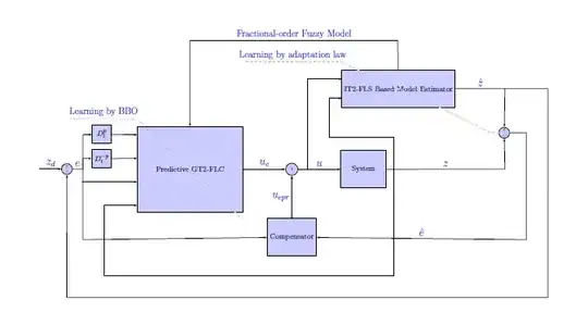
I have written a code for my block diagram as shown below:

enter image description here

\documentclass[10pt]{article}
\usepackage{adjustbox}
\usepackage{tikz}
\usetikzlibrary{plotmarks,matrix,decorations.pathreplacing,arrows.meta,calc,chains,shapes.geometric,backgrounds,fit,arrows,positioning}

\tikzset{ block/.style={ draw, fill=blue!20, rectangle, minimum height=5em, minimum width=6em }, every label/.append style = {text= blue, align=center}, blockk/.style={ draw, fill=blue!20, rectangle, minimum height=2.5em, minimum width=2.5em }, blockkk/.style={ draw, fill=blue!20, rectangle, minimum height=11.3em, minimum width=14em }, sum/.style={ draw, fill=blue!20, circle, minimum size=0.5cm, }, input/.style={coordinate}, output/.style={coordinate}, pinstyle/.style={pin edge={to-,thin,black}} }

\begin{document} \begin{figure*} \begin{adjustbox}{width=\textwidth,height=\textheight,keepaspectratio} \begin{tikzpicture}[auto,>=latex'] % We start by placing the blocks \node [input, name=input] {}; \node [sum, right = of input] (sum) {}; \node [blockk, above right = of sum] (derivative) {$D_t^p$}; \node [blockk, below = 0.25cm of derivative] (integral) {$D_t^{-p}$}; \node [blockkk, below right = -0.8cm and 1.2cm of derivative] (controller) {Predictive GT2-FLC}; \node [sum, right = 2cm of controller] (sum1) {\tiny+}; \node [block, right = 2cm of sum1] (system) {System}; \node [block, below = 2cm of sum1] (compensator) {Compensator}; \node [block, above right = 2cm and -2.1cm of system] (estimator) {IT2-FLS Based Model Estimator}; \node [sum, below right = 1cm and 2.1cm of estimator] (sum2) {}; \node[above=-2pt] at (sum.center){\tiny $+$}; \node[below=-2pt] at (sum.center){\tiny $-$}; \node[above=-2pt] at (sum2.center){\tiny $+$}; \node[below=-2pt] at (sum2.center){\tiny $-$};

\draw [draw,->] (input) -- node {\textcolor{blue}{\Large $z_d$}} (sum); %input
\draw [draw,->] (sum) -- node {\textcolor{blue}{\Large $e$}} (+2cm,0)--(+2cm,+1.6cm)--(derivative); %derivative
\draw [draw,->] (+2cm,0.5)--(integral); % e to integral
\draw [draw,->] (derivative) -- (4.55,1.6); %integral to controller
\draw [draw,->] (integral) -- (4.55,0.5);%derivative to controller
\draw [draw,->] (2,-0.6)--(4.55,-0.6); %e to controller
\draw[double,dashed,-](sum2)--(21,1.7)-- ([yshift=-1em]estimator.south east) -- ([yshift=1em]estimator.north west)--node[above]{\textcolor{blue}{\large Learning by adaptation law}}(9.5,5);
\draw [draw,->] (controller) -- node {\textcolor{blue}{\Large $u_c$}} (sum1); %controller to sum1
\draw [draw,->] (compensator) -- node {\textcolor{blue}{\Large $u_{cpr}$}} (sum1); %sum1 to compensator
\draw [draw,->] (+2cm,0.5)--(+2,-3.3)--(compensator);%e to compensator
\draw [draw,->] (sum1) -- node {\textcolor{blue}{\Large $u$}} (system); %sum1 to system
\draw [draw,->] (12.5,-0)--(12.5,4.2)--(14.1,4.2); %u to estimator
\draw [draw,<->] (4.55,-1.7)->(3,-1.7)--(3,-5)--(16.5,-5)--(16.5,1.5)--(13.5,1.5)--(13.5,3.3)->(14.1,3.3); %controller to estimator
\draw [draw,->] (estimator) -- (+16.7cm,6)--node[above]{\textcolor{blue}{\large Fractional-order Fuzzy Model}}(7,6)--(controller); %estimator to controller
\draw [draw,->] (estimator)--node {\textcolor{blue}{\Large $\hat{z}$}} (21.7,3.75)--(sum2); %estimator to sum2
\draw [draw,->] (21.7,3.75)--(23.7,3.75)--(23.7,-6)--(1.25,-6)--(sum); %yhat to sum
\draw [draw,->] (system)-- node {\textcolor{blue}{\Large $z$}} (21.7,0)-- (sum2); %system to sum2
\draw [draw,->] (sum2) --(22.7,1.7)--(22.7,-3.3)--node[above]{\textcolor{blue}{\Large $\hat{e}$}} (compensator); %sum2 to compensator
\draw[double,dashed,-] ([yshift=-1em]controller.south east) -- ([yshift=1em]controller.north west)--node[above] {\textcolor{blue}{\large Learning by BBO}}(1.4,2.35);

\end{tikzpicture} \end{adjustbox} \end{figure*} \end{document}

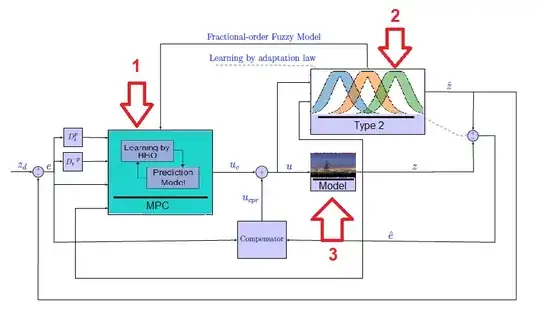
Now, I want to make some changes as shown by the arrows in this picture:

enter image description here

Arrow 1- to make it look as shown, doing it entirely with coding

Arrow 2- to make it look as shown, doing it entirely with coding

Arrow 3- to make it look as shown using an image. use an arbitrary 120*120 (pixels) image
Milito
  • 45
  • 2
    Sorry, I must have missed something but where are the three arrows you're mentioning? I suppose they're on the three blocks but could you be more precise? – SebGlav Jul 29 '23 at 12:55
  • Looks nice. Unfortunately your code can‘t compile. Please add the missing parts. Thank you – MS-SPO Jul 29 '23 at 13:21
  • 1
    Sorry, I added the missing part. Now the code can be compiled. I also added the three arrows to the picture. – Milito Jul 29 '23 at 14:16
  • Thank you. Unfortunately a few things still are missing: your code should a) start with documentclass, b) end with end{document}, c) still show your situation after compile. Thank you – MS-SPO Jul 29 '23 at 14:38
  • 1
    documentclass is added. – Milito Jul 29 '23 at 14:51
  • What's the issue with (1) exactly? Isn't that just more of the kind of thing you've got already i.e. a couple of blocks with arrows? For (2) you could always compile an image and then include it. Or you could code it in-place, though I'm not sure whether it is meant to be something specific. What's the problem with (3)? – cfr Jul 29 '23 at 16:03
  • I suggest to leave this question open, as all you need to know is present meanwhile, in my view. – MS-SPO Jul 29 '23 at 16:28

2 Answers2

2

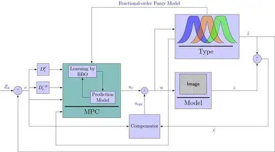
The rectangles around other stuff can be achieved with a matrix (unless you need to transform this rectangle in some shape or form).

With the generate anchors solution from a recent answer we create a bunch of anchors on the left side of every node which we can use to reference a position of other nodes or connect lines to it.

The ext.paths.ortho library provides various orthogonal connections, the ext.positioning-plus library makes it a bit easier to find a coordinate in reference to multiple other nodes.

I provide a subtitle pic that places a thick line and a node below something else. I'm not sure how long this line should be because in your sketch it is sometimes longer and sometimes short than what's above it.

Code

\documentclass[tikz]{standalone}
\usetikzlibrary{arrows.meta, calc, ext.paths.ortho, ext.positioning-plus, graphs, quotes}
\makeatletter
\pgfset{
  @generate anchors/.code n args={4}{%
    \pgfmathloop\pgfmathparse{\pgfmathcounter/(#2+1)}%
      \pgfset{generate anchors/.expanded={#1 \pgfmathcounter/#2:\pgfmathresult}{#3}{#4}}%
      \ifnum\pgfmathcounter<#2\relax\repeatpgfmathloop},
  @generate anchor/.code args={#1:#2:#3:#4}{%
    \pgfdeclaregenericanchor{#1}{%
      \pgfpointlineattime{#2}{\pgf@sh@reanchor{##1}{#3}}{\pgf@sh@reanchor{##1}{#4}}}},
  generate anchors/.style n args={3}{
    /utils/tempa/.style={/pgf/@generate anchor={##1:#2:#3}}, /utils/tempa/.list={#1}}}
\makeatother
\pgfset{@generate anchors={in}{8}{north west}{south west}}
\tikzset{
  subtitle length/.initial=2cm,
  subtitle/.pic={
    \coordinate[below={.6666em of #1}] (@);
    \draw[shift=(@), ultra thick, pic actions] (left:\pgfkeysvalueof{/tikz/subtitle length})
                                           -- (right:\pgfkeysvalueof{/tikz/subtitle length})
      node[below, midway, node font=\Large, style/.expand once=\tikzpictextoptions]{\tikzpictext};},
  /utils/temp/.style n args={3}{% allow r-du, r-ud, r-lr, r-rl to be used inside to and edges
    #1#2/.style={to path={r-#1#2(\tikztotarget)\tikztonodes}},
    #1#2 through point/.style={to path={% udlr paths through a point
      let \p{start}=($(##1)-(\tikztostart)$), \p{target}=($(##1)-(\tikztotarget)$) in
      r-#1#2[#1#2 distance/.expanded={min(abs(#3{start}),abs(#3{target}))}, from center]
      (\tikztotarget)\tikztonodes}}},
  /utils/temp/.list={lr\x, rl\x, du\y, ud\y}}
\begin{document}
\begin{tikzpicture}[
  Block/.style args={#1x#2}{
    draw, fill=blue!20, shape=rectangle, align=center, minimum width={#1}, minimum height={#2}},
  block/.style ={Block =  0pt   x  0pt},
  block1/.style={Block =  6em   x  5em},
  block2/.style={Block =  2.5em x  2.5em},
  block3/.style={Block = 14em   x 11.3em},
  every edge quotes/.append style = {text=blue, align=center},
  sum/.style={
    draw, fill=blue!20, circle, minimum size=0.5cm, align=center, node font=\tiny},
  input/.style={coordinate},
%  output/.style={coordinate},
  auto, >=Latex, node distance=\nd, ortho/install shortcuts,
  up and down curve/.style={insert path={
      (0,0) coordinate (curve-start)
            to[out=30, in=180, in distance=3mm] ++(1, 2) -- ++(right:.5)
            to[out= 0, in=150, out distance=3mm] ++(1,-2)
         #1 ++(left:.2) coordinate (curve-end) [rounded corners]
            to[out=180, in=-80] ++(-1.05, 1.7) [sharp corners]
            to[out=260, in=0] (right:.2)}}
]
\newcommand*\nd{1cm}

\node [input] (input) {}; \node [sum, right = of input] (sum) {$+$\$-$}; \matrix[fill=teal!50, draw, right=3:of sum] (controller){ \node[block] (c1) {Learning by\BBO} node[block, below=of c1, xshift=1.5cm] (c2) {Prediction\Model}; \path[horizontal vertical, ->] (c1) edge (c2) (c2) edge (c1); \pic["MPC"] {subtitle=(c1)(c2)}; \}; \node [block2, left = of controller.in 1/8] (derivative) {$D_t^p$} edge[-*, ->] (controller); \node [block2, left = of controller.in 4/8] (integral) {$D_t^{-p}$} edge[-*, ->] (controller); \node[sum, right=1.5:of controller] (sum1) {$+$}; \node[block1, below=1.5:of sum1] (compensator) {Compensator}; \matrix[block, right=2:of sum1] (system) { \nodeinner sep=+0pt{\includegraphics[width=2cm, keepaspectratio]{example-image}}; \pic["Model", subtitle length=1.2cm] {subtitle=(c1)}; \}; \matrix[block, west above=of system] (estimator){ \foreach[count=\i from -1] \c in {blue, orange, green} \fill[\c, opacity=.5, shift=(right:\i), name suffix=\i, up and down curve=--] -- cycle; \foreach \i in {-1, 0, 1} \draw[shift=(right:\i), up and down curve=]; \pic["Type "]{subtitle=(curve-start-1)(curve-end1)}; \}; \node[sum, right=of estimator.south east] (sum2) {$+$\$-$};

\coordinate[below=.5:of compensator] (comp1); \coordinate[below=.5:of comp1] (comp2); \coordinate[right=of sum2] (sum21); \graph[use existing nodes] { input ->["$Z_d$"] sum ->[-|-, /tikz/ortho/distance=\nd/2] { derivative, integral, compensator, controller[> {"$e$" very near start, graphs/right anchor=in 6/8}]}, controller ->["$u_c$"] sum1 ->["$u$"] system ->["$z$" near start, -|] sum2 ->["$\hat e$" very near end, rl] compensator ->["$u_{\mathrm{epr}}$"] sum1 ->[-|-, /tikz/ortho/ratio=.25, right anchor=in 3/8] estimator ->["$\hat z$" near start, -|] sum2, estimator ->[ud, clear >, "Fractional-order Fuzzy Model"'] controller, estimator ->[left anchor=in 5/8, right anchor=in 8/8, to path={ --++(left:\nd/2) {to[du through point=comp1] ([shift=(left:\nd/2)]\tikztotarget)} -- (\tikztotarget)}] controller, estimator ->[to path={-| (sum21) |- (comp2) -| (\tikztotarget)}] sum }; \end{tikzpicture} \end{document}

Output

enter image description here

Qrrbrbirlbel
  • 119,821
0

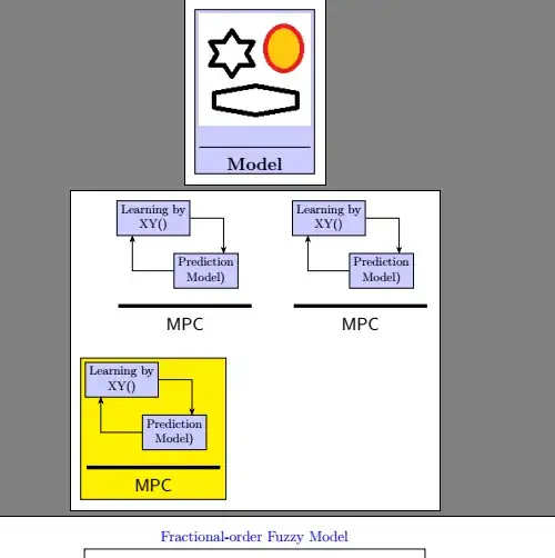
Here are some ways to do it.

General:

  • for development it's easier to use standalone
  • so \figure and adjustbox aren't needed here
  • package graphicx lets you include images

Save as icon.png:

icon

Main ideas for arrow 3:

  • treat as LaTeX-text inside the nodes { }
  • so \includegraphics
  • use \\ for new lines, together with align=center
  • use \hrulefill for the rule

Main ideas for arrow 1:

  • introduced a pic-style named mpc via \tikzset{}
  • it places boxes, line and text manually (by eye in my case)
  • call \pic {}; like you would call nodes, specify the style as {mpc};
  • place as many of thes \pics as you like
  • as node-text accept LaTeX inside the {}, {\tikz{..};}; is a valid argument
  • it was easiest to set the fill-color in said node
  • you can also scale pics, but you need to check on the transform option to avoid ... well, you'll see

Arrow 2 ...

you can build in a similar way. Look for cycle to close a path. Look for ways to bend linear lines in the manual. Look for transparency for the overlapping parts.

With this in mind you should be able to adjust your drawing.

results

%\documentclass[10pt]{article}
\documentclass[10pt,border=3mm,tikz]{standalone}% better for development
%\usepackage{adjustbox}% then this one is not needed
\usepackage{tikz}
\usetikzlibrary{plotmarks,matrix,decorations.pathreplacing,
                arrows.meta,calc,chains,shapes.geometric,
                backgrounds,fit,arrows,positioning}
\usepackage{graphicx}% for the image

\tikzset{ block/.style={ draw, fill=blue!20, rectangle, minimum height=5em, minimum width=6em }, every label/.append style = {text= blue, align=center}, blockk/.style={ draw, fill=blue!20, rectangle, minimum height=2.5em, minimum width=2.5em }, blockkk/.style={ draw, fill=blue!20, rectangle, minimum height=11.3em, minimum width=14em }, sum/.style={ draw, fill=blue!20, circle, minimum size=0.5cm, }, input/.style={coordinate}, output/.style={coordinate}, pinstyle/.style={pin edge={to-,thin,black}} }

\begin{document}

% ~~~ arrow 3 ~~~~~~~~~~~~~~~~~~~~~~~~~~~~~~~~ \begin{tikzpicture} \node[align=center,% for multiline font={\Large\bfseries},% if you want larger fonts; the old bold-definition works fill=blue!20,% background; make image transparent with a paint program, if needed draw, ] {\includegraphics[scale=1]{icon}\ \hrulefill\ Model}; \end{tikzpicture}

% ~~~ arrow 1 ~~~~~~~~~~~~~~~~~~~~~~~~~~~~~~~~ \tikzset{ bx/.style={align=center, draw, fill=blue!20}, > = {Stealth}, tx/.style={font={\Large\bfseries\sf}},% if you prefer san serif % mpc/.pic={ % ~~~ blocks ~~~~~~~~~~~~~~~~ \node[bx] (A) {Learning by\XY()}; \node[bx] (B) at (1.5,-1.5) {Prediction\Model)}; % ~~~ connectors ~~~~~~~~~~~~~~ \draw [->] (A.east) -| (B.45);% anchor point in polar coordinates \draw [->] (B.west) -| (A.220); % ~~~ rest ~~~~~~~~~~~~ \node[tx] at (0.9,-3) {MPC}; \draw[line width=3pt] (-1,-2.5) -- +(3.8,0);% relative move } } % ~~~ now using said pic ~~~~~~~~~~ \begin{tikzpicture} \pic {mpc}; % place like nodes; type of pic inside the { } \pic at (5,0) {mpc}; \node[draw,fill=yellow] at (0,-6) {\tikz{\pic {mpc};}};% LaTeX inside { } \end{tikzpicture}

%\begin{figure*} %\begin{adjustbox}{width=\textwidth,height=\textheight,keepaspectratio} \begin{tikzpicture}[auto,>=latex'] % We start by placing the blocks \node [input, name=input] {}; \node [sum, right = of input] (sum) {}; \node [blockk, above right = of sum] (derivative) {$D_t^p$}; \node [blockk, below = 0.25cm of derivative] (integral) {$D_t^{-p}$}; \node [blockkk, below right = -0.8cm and 1.2cm of derivative] (controller) {Predictive GT2-FLC}; \node [sum, right = 2cm of controller] (sum1) {\tiny+}; \node [block, right = 2cm of sum1] (system) {System}; \node [block, below = 2cm of sum1] (compensator) {Compensator}; \node [block, above right = 2cm and -2.1cm of system] (estimator) {IT2-FLS Based Model Estimator}; \node [sum, below right = 1cm and 2.1cm of estimator] (sum2) {}; \node[above=-2pt] at (sum.center){\tiny $+$}; \node[below=-2pt] at (sum.center){\tiny $-$}; \node[above=-2pt] at (sum2.center){\tiny $+$}; \node[below=-2pt] at (sum2.center){\tiny $-$};

% ~~~ connections ~~~~~~~~~~~~~~~~~~~~~~~~~~~~~~~~~~~~~~~~~~~~~~~~~
\draw [draw,-&gt;] (input) -- node {\textcolor{blue}{\Large $z_d$}} (sum); %input
\draw [draw,-&gt;] (sum) -- node {\textcolor{blue}{\Large $e$}} (+2cm,0)--(+2cm,+1.6cm)--(derivative); %derivative
\draw [draw,-&gt;] (+2cm,0.5)--(integral); % e to integral
\draw [draw,-&gt;] (derivative) -- (4.55,1.6); %integral to controller
\draw [draw,-&gt;] (integral) -- (4.55,0.5);%derivative to controller
\draw [draw,-&gt;] (2,-0.6)--(4.55,-0.6); %e to controller
\draw[double,dashed,-](sum2)--(21,1.7)-- ([yshift=-1em]estimator.south east) -- ([yshift=1em]estimator.north west)--node[above]{\textcolor{blue}{\large Learning by adaptation law}}(9.5,5);
\draw [draw,-&gt;] (controller) -- node {\textcolor{blue}{\Large $u_c$}} (sum1); %controller to sum1
\draw [draw,-&gt;] (compensator) -- node {\textcolor{blue}{\Large $u_{cpr}$}} (sum1); %sum1 to compensator
\draw [draw,-&gt;] (+2cm,0.5)--(+2,-3.3)--(compensator);%e to compensator
\draw [draw,-&gt;] (sum1) -- node {\textcolor{blue}{\Large $u$}} (system); %sum1 to system
\draw [draw,-&gt;] (12.5,-0)--(12.5,4.2)--(14.1,4.2); %u to estimator
\draw [draw,&lt;-&gt;] (4.55,-1.7)-&gt;(3,-1.7)--(3,-5)--(16.5,-5)--(16.5,1.5)--(13.5,1.5)--(13.5,3.3)-&gt;(14.1,3.3); %controller to estimator
\draw [draw,-&gt;] (estimator) -- (+16.7cm,6)--node[above]{\textcolor{blue}{\large Fractional-order Fuzzy Model}}(7,6)--(controller); %estimator to controller
\draw [draw,-&gt;] (estimator)--node {\textcolor{blue}{\Large $\hat{z}$}} (21.7,3.75)--(sum2); %estimator to sum2
\draw [draw,-&gt;] (21.7,3.75)--(23.7,3.75)--(23.7,-6)--(1.25,-6)--(sum); %yhat to sum
\draw [draw,-&gt;] (system)-- node {\textcolor{blue}{\Large $z$}} (21.7,0)-- (sum2); %system to sum2
\draw [draw,-&gt;] (sum2) --(22.7,1.7)--(22.7,-3.3)--node[above]{\textcolor{blue}{\Large $\hat{e}$}} (compensator); %sum2 to compensator
\draw[double,dashed,-] ([yshift=-1em]controller.south east) -- ([yshift=1em]controller.north west)--node[above] {\textcolor{blue}{\large Learning by BBO}}(1.4,2.35);

\end{tikzpicture} %\end{adjustbox} %\end{figure*} \end{document}

MS-SPO
  • 11,519
  • 2
    \tikz{} is NOT valid inside a tikzpicture environment. Nesting pictures isn't supported and leads to weird issues which aren't always obvious and can be difficult to pin down. This is why tikzmarks, for example, uses different mechanisms inside tikzpictures. What you could do is save the \tikz{} to a box and then use the box in the node. That would be much safer. – cfr Jul 29 '23 at 19:30
  • 2
    Also, you shouldn't use two-letter font macros such as \sf in LaTeX. Try \sffamily instead. – cfr Jul 29 '23 at 19:33
  • @cfr, thank you for your comments. – MS-SPO Jul 29 '23 at 19:53
  • 1
    @MS-PSO thank you – Milito Aug 01 '23 at 12:51