8

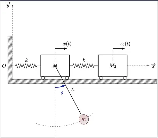
I am new with Tikz and I managed to combine several Tikz code samples [x] to represent a 3-degree of freedom system. However, I would like to 'translate'/move the pendulum from mass M to the second mass M2 but it doesn't work. The center of the pdf content seems to be defined at the M.center and the "definition" of angle as well. I did not achieve to change that as I tried to move the pendulum, the angle won't translate to the next mass M2.

See the code below:

\documentclass[tikz]{standalone}
\usetikzlibrary{calc,patterns,decorations.pathmorphing,decorations.markings}

\usepackage{physics} \usepackage{siunitx} \sisetup{detect-all} % to allow \pi in \SI \usepackage{tikz,pgfplots} \usepackage[outline]{contour} % glow around text \usetikzlibrary{calc} \usetikzlibrary{angles,quotes} % for pic \usetikzlibrary{arrows.meta} \tikzset{>=latex} % for LaTeX arrow head \contourlength{1.2pt}

\colorlet{xcol}{blue!70!black} \colorlet{vcol}{green!60!black} \colorlet{myred}{red!70!black} \colorlet{myblue}{blue!70!black} \colorlet{mygreen}{green!70!black} \colorlet{mydarkred}{myred!70!black} \colorlet{mydarkblue}{myblue!60!black} \colorlet{mydarkgreen}{mygreen!60!black} \colorlet{acol}{red!50!blue!80!black!80} \tikzstyle{CM}=[red!40!black,fill=red!80!black!80] \tikzstyle{xline}=[xcol,thick,smooth] \tikzstyle{mass}=[line width=0.6,red!30!black,fill=red!40!black!10,rounded corners=1,top color=red!40!black!20,bottom color=red!40!black!10,shading angle=20] \tikzstyle{faded mass}=[dashed,linewidth=0.1,red!30!black!40,fill=red!40!black!10,rounded corners=1,top color=red!40!black!10,bottom color=red!40!black!10,shading angle=20] \tikzstyle{rope}=[black!70!black,thick,line cap=round] \def\rope#1{ \draw[black,line width=0.8] #1; \draw[rope,line width=1.1] #1; } \tikzstyle{force}=[->,myred,very thick,line cap=round] \tikzstyle{velocity}=[->,vcol,very thick,line cap=round] \tikzstyle{Fproj}=[force,myred!40] \tikzstyle{myarr}=[-{Latex[length=3,width=2]},ultra thick] \def\tick#1#2{\draw[thick] (#1)++(#2:0.12) --++ (#2-180:0.24)} \DeclareMathOperator{\sn}{sn} \DeclareMathOperator{\cn}{cn} \DeclareMathOperator{\dn}{dn} \def\N{80} % number of samples in plots

\tikzstyle{axis}=[->,thick] %line width=0.6

%%%%%%%%%%%%%%%%%%%%%%%%%%%%%%%%%%%%%%%%%%%%%%%%%%%%%%%%%%%%%%%%%%%%%%%%%%%%%% %%%%%%%%%%%%%%%%%%%%%%%%%%%%%%%%%%%%%%%%%%%%%%%%%%%%%%%%%%%%%%%%%%%%%%%%%%%%%% \tikzstyle{spring}=[thick,decorate,decoration={zigzag,pre length=0.3cm,post length=0.3cm,segment length=6,amplitude=1.75mm}] %amplitude=1.75mm \tikzstyle{damper}=[thick,decoration={markings,
mark connection node=dmp, mark=at position 0.5 with { \node (dmp) [thick,inner sep=0pt,transform shape,rotate=-90,minimum width=15pt,minimum height=3pt,draw=none] {}; \draw [thick] ($(dmp.north east)+(2pt,0)$) -- (dmp.south east) -- (dmp.south west) -- ($(dmp.north west)+(2pt,0)$); \draw [thick] ($(dmp.north)+(0,-5pt)$) -- ($(dmp.north)+(0,5pt)$); } }, decorate] \tikzstyle{ground}=[fill,pattern=north east lines,draw=none,minimum width=0.75cm,minimum height=0.3cm,inner sep=0pt,outer sep=0pt]

\definecolor{monOrange}{RGB}{255,157,0} \definecolor{monBleu}{rgb}{0.2,0.4,0.6} \definecolor{monCyan}{RGB}{74,181,247} \definecolor{monGris}{RGB}{100,100,100} \definecolor{monRed}{RGB}{255, 36, 0}

\tikzset{ seisme/.style={color=cyan,ultra thick,->}, vent/.style={color=monRed,ultra thick,->}, }

%%%%%%%%%%%%%%%%%%%%%%%%%%%%%%%%%%%%%%%%%%%%%%%%%%%%%%%%%%%%%%%%%%%%%%%%%%%%%% %%%%%%%%%%%%%%%%%%%%%%%%%%%%%%%%%%%%%%%%%%%%%%%%%%%%%%%%%%%%%%%%%%%%%%%%%%%%%% \begin{document}

%%%%%%%%%%%%%%% SHEMA MODAL 3DDL %%%%%%%%%%%%%%% \begin{tikzpicture}[scale=1.1, every node/.style={scale=1.3}] % Rectangle masse m1 + petites roues \node [draw, outer sep=0pt, thick] (M) [minimum width=2cm, minimum height=1.5cm] {$M$}; \draw [thick, fill=white] (M.south west) ++(0.2cm,-0.125cm) circle (0.125cm) (M.south east) ++(-0.2cm,-0.125cm) circle (0.125cm);

% Rectangle masse m2 + petites roues \node [draw, outer sep=0pt, thick] (M2) [minimum width=2cm, minimum height=1.5cm, xshift = 4cm] {$M_2$}; % rectangle entourant la masse m2 \draw [thick, fill=white] (M2.south west) ++(0.2cm,-0.125cm) circle (0.125cm) (M2.south east) ++(-0.2cm,-0.125cm) circle (0.125cm); % 2 petits cercles sous la masse m2

% Ground bas \node (ground) [ground,anchor=north,yshift=-0.2cm,minimum width=10cm,xshift=2.03cm] at (M.south) {}; % ground bas hachurage \draw (ground.north west) -- (ground.north east) -- (ground.south east) -- (ground.south west); %traits horizontaux entourant le ground bas \node (fill) [ground,xshift=-0.15cm,minimum height = 0.3cm, minimum width = 0.3cm] at (ground.west) {}; %petit ajout de ground bas tout à gauche \draw (fill.north west) -- (fill.south west) -- (fill.south east);

% Ground vertical \node (wall) [ground, rotate=-90, minimum width=3cm,anchor=south east] at (fill.north west) {}; % ground vertical hachurage \draw (wall.north east) -- (wall.north west) -- (wall.south west) -- (wall.south east); %traits horizontaux entourant le ground vertical

% % Ressort k \draw [spring] (M.east) -- (M2.west) node (k) [midway,yshift=0.4cm] {$k$};

% Ressort k \draw [spring] (wall.15) node[left= 0.3cm]{$O$} -- ($(M.north west)!(wall.15)!(M.south west)$) node [midway,yshift=0.4cm] {$k$};

% Force d'excitation sur la masse m2 %\draw [-latex,ultra thick] (M2.east) -- +(1cm,0cm) node [right] (u) {$F(t) = F_0 \sin{\omega t}$};

%Déplacement de la masse m1 noté y1 \draw [-latex,ultra thick] (M.center) ++(0cm, 1.4cm) -- +(1cm,0cm) node [above] (y1) {$x(t)$}; % flèche déplacement x(t) \draw [dashed] (M.center) -- +(0cm,1.4cm); % trait pointillés y1

% Déplacement de la masse m2 noté y2 \draw [-latex,ultra thick] (M2.center) ++(0cm, 1.4cm) -- +(1cm,0cm) node [above] (y2) {$x_2(t)$}; % flèche déplacement x(t) \draw [dashed] (M2.center) -- +(0cm,1.4cm); % trait pointillés y2

% Axes (x,y) et centre 0 du repère cartésien %\draw[axis] (0,0)--(5.7,0) node[right] {$\overrightarrow{x}$} \drawdashed,->--(7.7,0) node[right]{$\overrightarrow{x}$}; \drawdashed,->--(-3.5,5) node[left]{$\overrightarrow{y}$};

% PENDULUM \def\L{5} % string length \def\ang{28} % angle string \def\R{0.4} % ball radius \def\F{1.0} % force magnitude \coordinate (M) at (\ang-90:\L); \coordinate (M') at (0,-\L); \coordinate (O) at (0,0); \coordinate (B) at (0,-\L-2.2\R); \coordinate (FT) at ($(M)+(90+\ang:{\Fcos(\ang)+\R})$); \coordinate (FG) at ($(M)+(-90:{\F+\R})$); \coordinate (FGx) at ($(M)+(-90+\ang:{0.55\F+\R})$); \coordinate (MA) at ($(M)+(180+\ang:{\Fsin(\ang)+\R})$); %\draw[faded mass] (M') circle(\R); \draw[dashed] (O) -- (B); \draw[dashed] (-90+\ang+10:\L) arc(-90+\ang+10:-110:\L) (B); \rope{(O) -- (M)} \path (O) -- (M) node[midway,above right=-1] {$L$}; \fill[black] (O) circle(0.04); \draw[mass] (M) circle(\R) node {$m$}; \draw pic[myarr,"$\theta$",xcol,draw=xcol,angle radius=43,angle eccentricity=1.30] {angle=B--O--M};

\end{tikzpicture}

\end{document}

Here is what I get: 3-degree of freedom system

Any sugestion would be welcome!

Pendulum TikZ code source

Ground-mass-spring system code source

AlexG
  • 54,894
Ben
  • 81
  • 1
    Welcome to TeX.SX! The pgfplots package loads tikz, but requires to set the compat option. Do you need pgfplots at all? You should use \tikzset instead of \tikzstyle. Also, you should probably not (re)define short commands like \N in the global scope. – Jasper Habicht Dec 21 '23 at 10:03
  • 1
    Please include links to the sources for the code you've used. This makes it easy to find the context if people need/want it. – cfr Dec 21 '23 at 15:30
  • 1
    Don't you get an error with this code? It doesn't compile for me .... – cfr Dec 21 '23 at 15:33
  • 1
    @cfr You are right, I did forget the first two lines of the code! (\documentclass and \usetikzlibrary). I edited it and the code does compile now. I also added the links to the source code which I used as you suggested. – Ben Dec 21 '23 at 17:20
  • @Ben, from a systematic point of view you could summarize some code parts into one or more \pic statements, see https://tikz.dev/tikz-pics . Think of the as macros for Tikz. – MS-SPO Dec 21 '23 at 17:30
  • 1
    Thanks for editing. That's definitely helpful. You could use pics as @MS-SPO suggested, but I'm not sure I'd recommend it if you've just started using TikZ. pics have some idiosyncrasies which may just introduce unnecessary confusion at this point. Better, I think, to work through the tutorials at the start of the TikZ manual first and draw some simple pictures with basic building blocks so you get a 'feel' for how things work first. – cfr Dec 21 '23 at 17:37

2 Answers2

16

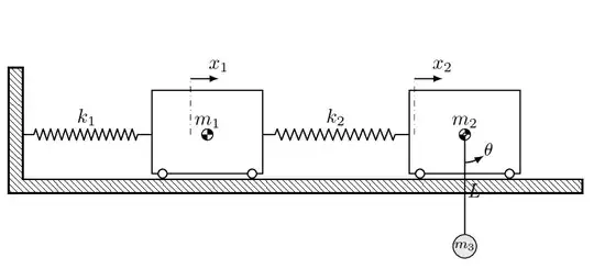
For fun, the animated simulation result.

The equations of motion have been derived from the system's kinetic and potential energies by means of the Lagrange formalism and solved with \pstODEsolve from package pst-ode. enter image description here enter image description here

%\documentclass[margin=3pt,10pt,export]{standalone} % for GIF
%\documentclass[margin=3pt,10pt,dvisvgm]{standalone} % for SVG, run twice: dvilualatex example ; dvisvgm --font-format=woff --zoom=-1 --page=1 example.dvi
\documentclass[margin=3pt,10pt]{standalone} % for PDF, run lualatex twice

\usepackage{pst-ode} \usepackage[loop,controls]{animate} \usepackage{tikz} \usetikzlibrary{calc,arrows.meta,decorations.pathmorphing,patterns.meta} \usepackage{listofitems} % read space separated items \usepackage[T1]{fontenc} \usepackage{xsavebox}

% adjustable parameters & definitions \pstVerb{ tx@Dict begin % all definitions within PSTricks dict /tEnd 60 def % time span to be simulated [s] % /tEnd 13.56 def % this time span gives a nearly cyclic impression, suitable for GIF /m1 1 def % mass_1 [kg] /m2 1 def % mass_2 [kg] /m3 0.1 def % mass_3 (bob) [kg] /L 2 def % pendulum length [m] /k1 80 def % spring constant [kg/s^2] /k2 40 def % spring constant [kg/s^2] /g 9.81 def % acceleration [m/s^2] /x2Zero 0.9 def % initial displacement of mass_2 [m] /thetaZero 0 def % initial displacement of pendulum from vertical [°] %
% (integer) number of time steps (for 25 frames per s) + 1 /N (cvi(tEnd25+1)) AlgParser cvx exec def % % initial displacement of mass_1 /x1Zero (k2/(k1+k2)x2Zero) AlgParser cvx exec def % % some constants /k12M1 ((k1+k2)/m1) AlgParser cvx exec def /k2M1 (k2/m1) AlgParser cvx exec def % % displacements of mass_1, mass_2, pendulum /x1 (x[0]) AlgParser cvx def /x2 (x[1]) AlgParser cvx def /theta (x[2]) AlgParser cvx def % %%%%%%%%%%%%%%%%%%%%%%%%%%%%%%%%%%%%%%%%%%%%% % 1st order ODE system (equations of motion) %%%%%%%%%%%%%%%%%%%%%%%%%%%%%%%%%%%%%%%%%%%%% % velocities /v1 (x[3]) AlgParser cvx def /v2 (x[4]) AlgParser cvx def /omega (x[5]) AlgParser cvx def % accelerations /a1 (k2M1x2 - k12M1x1) AlgParser cvx def /a2 ((m3sin(theta)(gcos(theta)+Lomega^2)-k2(x2-x1))/(m2+m3sin(theta)^2)) AlgParser cvx def /alpha (-(a2cos(theta) + gsin(theta))/L) AlgParser cvx def end }

% solve equations of motion \pstODEsolve[algebraicAll,saveData]{timeX1X2Theta}{ % PS variable and file (base-)name that take result list t | x1 | x2 | RadtoDeg(theta-TwoPi*cvi(theta/TwoPi)) % table format of data to be saved in timeX1X2Theta(.dat) }{0}{tEnd}{N}{ % t_0, t_end, number of time steps + 1 x1Zero | x2Zero | DegtoRad(thetaZero) | 0 | 0 | 0 % initial conditions (displacements, velocities) }{ v1 | v2 | omega | a1 | a2 | alpha % ODE system's RHS }

%%%%%%%%%%%%%%%%%%%%%%%%%%%%%%%%%%%%%%%%%%%%%%%%%%%%%%%%%%%%%%%%%%%%%%%%%%%%%%%%% % \fileopenr{<file stream>}{<file name>}, opens file for reading \newcommand\fileopenr[2]{% \newread#1% \immediate\openin#1=#2% } % \readtolist[<sep char>]{<file stream>}{\list} % reads a line from file stream and splits at <sep char> into \list[1], \list[2], ... \newcommand\readtolist[3][,]{{% \setsepchar{#1}% \immediate\read#2 to \inputline% \ifeof#2 \immediate\closein#2% \ifdefined\multiframebreak\multiframebreak\fi% \else% \greadlist*#3\inputline% \fi% }} %%%%%%%%%%%%%%%%%%%%%%%%%%%%%%%%%%%%%%%%%%%%%%%%%%%%%%%%%%%%%%%%%%%%%%%%%%%%%%%%%

\tikzset{spring/.style={decorate, decoration={zigzag,pre length=0.2cm,post length=0.2cm,segment length=\dimexpr(#1-0.4cm-1pt)/14\relax, amplitude=0.1cm}}}

\begin{document} \IfFileExists{timeX1X2Theta.dat}{}{dummy\end{document}}% % cart \begin{xlrbox}{cart} \begin{tikzpicture}[line width=0.2mm] \useasboundingbox (-1,0) rectangle (1,1.6); \draw (-0.99,0.1) rectangle (0.99,1.59); \fill [radius=0.1] (0,0.8) -- ++(0.1,0) arc [radius=0.1,start angle=0,end angle=90] -- ++(0,-0.2) arc [start angle=270, end angle=180]; \draw [thin] (0,0.8) circle [radius=0.1]; \filldraw [fill=white] (-0.8,0.1) circle [radius=0.08] (0.8,0.1) circle [radius=0.08]; \end{tikzpicture} \end{xlrbox}% % \begin{animateinline}{25} \fileopenr{\data}{timeX1X2Theta.dat}% \readtolist[ ]{\data}{\table}% \multiframe{10000}{}{ \begin{tikzpicture}[line width=0.2mm] \useasboundingbox (-0.3,-1.5) rectangle (10.1,3.1); % ground & wall \draw [pattern={Lines[angle=-45,line width=0.2pt,distance={3pt/sqrt(2)}]}] (0,0) -- (10,0) -- (10,-0.25) -- (-0.25,-0.25) -- (-0.25,2) -- (0,2) --cycle;
% cart 1 \path [shift={(\table[2],0)}] (3,0.8) node[inner sep=0, name={cart1}] {\thecart} node [anchor=south] {$m_1$}; % mass_2 (cart2) and mass_3 (bob) centres \path[shift={(\table[3],0)}] (7,0.8) coordinate (mass2) ++(\fpeval{\table[4]-90.0}:2) coordinate (bob); % cart 2 \path (mass2) node[inner sep=0] (cart2) {\thecart} node [anchor=south] {$m_2$}; % springs \coordinate (wall) at (0,0.8); \draw[line join=round, line cap=rect] let \p1=($(cart1.west)-(wall)$) in [draw,spring={\x1}] (wall) -- (cart1.west) node [midway,above,yshift=1pt] {$k_1$}; \draw[line join=round, line cap=rect] let \p1=($(cart2.west)-(cart1.east)$) in [draw,spring={\x1}] (cart1.east) -- (cart2.west) node [midway,above,yshift=1pt] {$k_2$}; % pendulum \draw (mass2) -- (bob) node[inner sep=1pt,midway,anchor=west,rotate={\table[4]}] {$L$}; \draw [thin,fill=white] (mass2) circle [radius=0.03]; \draw [thin,fill=white!90!black] (bob) circle [radius=0.21]; \path (bob) node[rotate={\table[4]}] {\scriptsize $m_3$}; % coordinates \draw[very thin,dashdotted] (3,0.8) -- ++(0,1); \draw[-latex] (3,0.8) ++(0,1) -- ++(0.5,0) node[above] {$x_1$}; \draw[very thin,dashdotted] (7,0.8) -- ++(0,1); \draw[-latex] (7,0.8) ++(0,1) -- ++(0.5,0) node[above] {$x_2$}; \draw[very thin,dashdotted] (mass2) -- ++(0,-0.55); \draw[-latex] (mass2) ++(0,-0.5) arc [radius=0.5,start angle=270,end angle=300] -- ++(30:0.1) node[inner sep=0pt,above right] {\small $\theta$}; \end{tikzpicture}% \readtolist[ ]{\data}{\table} } \end{animateinline} \end{document}

AlexG
  • 54,894
  • 1
    This masterpiece needs both annotations of x1 and x2 to move with their respective masses. This multibody dynamics simulation is class. – Diaa Jan 07 '24 at 21:39
  • 1
    After a second look at the code logic, I found another gem which is the ability to consider all the system nonlinearities in the 1st order ODEs without the need to linearize them. Delicious :) – Diaa Jan 07 '24 at 21:46
  • 1
    très belle utilisation de pstOde associé à Tikz – rpapa Jan 08 '24 at 09:17
  • Merci! J'aimerais bien utiliser PSTricks pour le dessin aussi, afin d’éviter d'écrire et de lire le fichier externe. Pourtant, mes connaissances de PSTricks sont un peu limitées. – AlexG Jan 08 '24 at 09:41
  • 1
    @Diaa : Thanks for you kind comments! As for your second one, it works as long as the eqs for acceleration do not mutually depend on each other. It was necessary to substitute, at some point of the derivation, the angular acceleration into the eq for the linear one of m2 in order to remove the implicit dependency of the latter on the former. One-way dependency (\dot{\omega} on \dot{v}_2), as in the present form, is OK. – AlexG Jan 10 '24 at 09:03
9

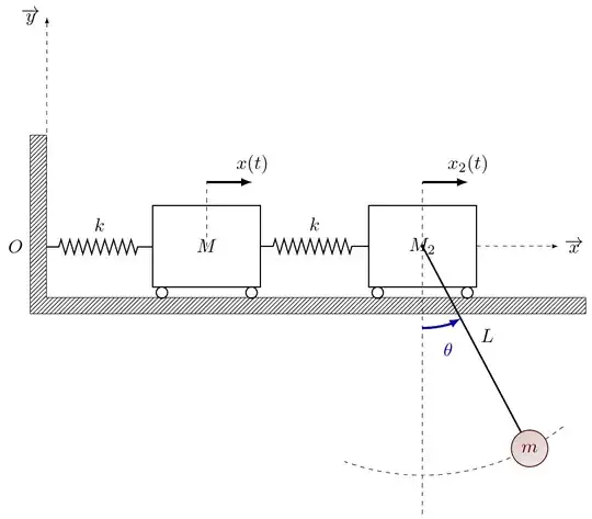
The simplest way is probably to just shift the pendulum code by (M2).

shifted pendulum

I partially cleaned up, minimised and updated your code, as well as fixing it to avoid the errors.

\documentclass[border=5pt]{standalone}
\usepackage{tikz}
\usetikzlibrary{calc,patterns,angles,quotes,arrows.meta,decorations.pathmorphing}
\tikzset{>=latex} % for LaTeX arrow head

\colorlet{xcol}{blue!70!black}

\tikzset{mass/.style={line width=0.6,red!30!black,fill=red!40!black!10,rounded corners=1,top color=red!40!black!20,bottom color=red!40!black!10,shading angle=20}} \tikzset{rope/.style={black!70!black,thick,line cap=round}} \tikzset{force/.style={->,myred,very thick,line cap=round}} \tikzset{myarr/.style={->,ultra thick}}

\newcommand\rope[1]{ \draw[black,line width=0.8] #1; \draw[rope,line width=1.1] #1; }

\tikzset{spring/.style={thick,decorate,decoration={zigzag,pre length=0.3cm,post length=0.3cm,segment length=6,amplitude=1.75mm}}, %amplitude=1.75mm damper/.style={thick,decoration={markings,
mark connection node=dmp, mark=at position 0.5 with { \node (dmp) [thick,inner sep=0pt,transform shape,rotate=-90,minimum width=15pt,minimum height=3pt,draw=none] {}; \draw [thick] ($(dmp.north east)+(2pt,0)$) -- (dmp.south east) -- (dmp.south west) -- ($(dmp.north west)+(2pt,0)$); \draw [thick] ($(dmp.north)+(0,-5pt)$) -- ($(dmp.north)+(0,5pt)$); } }, decorate}, ground/.style={fill,pattern=north east lines,draw=none,minimum width=0.75cm,minimum height=0.3cm,inner sep=0pt,outer sep=0pt}, }

\begin{document} %%%%%%%%%%%%%%% SHEMA MODAL 3DDL %%%%%%%%%%%%%%% \begin{tikzpicture}[scale=1.1, every node/.style={scale=1.3}] % Rectangle masse m1 + petites roues \node [draw, outer sep=0pt, thick] (M) [minimum width=2cm, minimum height=1.5cm] {$M$}; \draw [thick, fill=white] (M.south west) ++(0.2cm,-0.125cm) circle (0.125cm) (M.south east) ++(-0.2cm,-0.125cm) circle (0.125cm);

% Rectangle masse m2 + petites roues \node [draw, outer sep=0pt, thick] (M2) [minimum width=2cm, minimum height=1.5cm, xshift = 4cm] {$M_2$}; % rectangle entourant la masse m2 \draw [thick, fill=white] (M2.south west) ++(0.2cm,-0.125cm) circle (0.125cm) (M2.south east) ++(-0.2cm,-0.125cm) circle (0.125cm); % 2 petits cercles sous la masse m2

% Ground bas \node (ground) [ground,anchor=north,yshift=-0.2cm,minimum width=10cm,xshift=2.03cm] at (M.south) {}; % ground bas hachurage \draw (ground.north west) -- (ground.north east) -- (ground.south east) -- (ground.south west); %traits horizontaux entourant le ground bas \node (fill) [ground,xshift=-0.15cm,minimum height = 0.3cm, minimum width = 0.3cm] at (ground.west) {}; %petit ajout de ground bas tout à gauche \draw (fill.north west) -- (fill.south west) -- (fill.south east);

% Ground vertical \node (wall) [ground, rotate=-90, minimum width=3cm,anchor=south east] at (fill.north west) {}; % ground vertical hachurage \draw (wall.north east) -- (wall.north west) -- (wall.south west) -- (wall.south east); %traits horizontaux entourant le ground vertical

% % Ressort k \draw [spring] (M.east) -- (M2.west) node (k) [midway,yshift=0.4cm] {$k$};

% Ressort k \draw [spring] (wall.15) node[left= 0.3cm]{$O$} -- ($(M.north west)!(wall.15)!(M.south west)$) node [midway,yshift=0.4cm] {$k$};

% Force d'excitation sur la masse m2 %\draw [-latex,ultra thick] (M2.east) -- +(1cm,0cm) node [right] (u) {$F(t) = F_0 \sin{\omega t}$};

%Déplacement de la masse m1 noté y1 \draw [-latex,ultra thick] (M.center) ++(0cm, 1.4cm) -- +(1cm,0cm) node [above] (y1) {$x(t)$}; % flèche déplacement x(t) \draw [dashed] (M.center) -- +(0cm,1.4cm); % trait pointillés y1

% Déplacement de la masse m2 noté y2 \draw [-latex,ultra thick] (M2.center) ++(0cm, 1.4cm) -- +(1cm,0cm) node [above] (y2) {$x_2(t)$}; % flèche déplacement x(t) \draw [dashed] (M2.center) -- +(0cm,1.4cm); % trait pointillés y2

% Axes (x,y) et centre 0 du repère cartésien %\draw[axis] (0,0)--(5.7,0) node[right] {$\overrightarrow{x}$} \drawdashed,->--(7.7,0) node[right]{$\overrightarrow{x}$}; \drawdashed,->--(-3.5,5) node[left]{$\overrightarrow{y}$};

% PENDULUM \def\L{5} % string length \def\ang{28} % angle string \def\R{0.4} % ball radius \def\F{1.0} % force magnitude \begin{scope}[shift=(M2)] \coordinate (Mx) at (\ang-90:\L); \coordinate (M') at (0,-\L); \coordinate (O) at (0,0); \coordinate (B) at (0,-\L-2.2\R); \coordinate (FT) at ($(Mx)+(90+\ang:{\Fcos(\ang)+\R})$); \coordinate (FG) at ($(Mx)+(-90:{\F+\R})$); \coordinate (FGx) at ($(Mx)+(-90+\ang:{0.55\F+\R})$); \coordinate (MA) at ($(Mx)+(180+\ang:{\Fsin(\ang)+\R})$); \draw[dashed] (O) -- (B); \draw[dashed] (-90+\ang+10:\L) arc(-90+\ang+10:-110:\L) (B); \rope{(O) -- (Mx)} \path (O) -- (Mx) node[midway,above right=-1] {$L$}; \fill[black] (O) circle(0.04); \draw[mass] (Mx) circle(\R) node {$m$}; \draw pic[myarr,"$\theta$",xcol,draw=xcol,angle radius=43,angle eccentricity=1.30] {angle=B--O--Mx}; \end{scope} \end{tikzpicture}

\end{document}

cfr
  • 198,882
  • Wow thank you so much. I did try to "shift" manually the whole pendulum to (M2) but without success. I barely know how to use TikZ as you probably realized, so didn't know you could simply use the shift parameter this way. I needed to draw this model to illustrate my science project and did not take the time to properly study TikZ. Thank you for your time and the clean up of the code as it will help me get better to using TikZ. – Ben Dec 21 '23 at 17:29
  • @Ben You're welcome. Probably some of what I removed for the example you need for other diagrams, but the change to \tikzset{} you should use generally as \tikzstyle shouldn't be used in new documents. The shift combined with scope is a very useful trick ;). Note that I used Mx rather than M because you already had a node called M earlier and I found that confusing. – cfr Dec 21 '23 at 17:32