How to include result values in a LaTeX document?

Question

We are often in the following situation: a lengthy (data analysis) computation spits out a bunch of result values. Imagine a Python or script or an R script doing some resource intensive calculations. We then write an article or report, where we want to describe the results and list the result values in the text or in tables. Copy & pasting the values is error prone and a lo of work, so it would be good to automatically include the values.

Example: all numerical values here are results from scripts and need to be included in the article in some way or other:

What is the best way to achieve this?

Note: The computation might run for many hours - possible even on a separate computation cluster. Computing the results should therefore be a disentangled step from including the resultsin the LaTeX document and compiling it.

Bonus requirement: it might be nice to see the values displayed in the Latex editor (e.g. Overleaf) and not only the include command. This might be very helpful when using a Wysiwyg editor like the one on Overleaf, but I a doubt that one can do this without copy & pasting the values or preprocessing the Latex file somehow.

See also: this question on reddit.

Answer 1

Write results to separate text files and use \input

The most straight forward and simple solution is to write each value to a text file during the computation. The computation could, for example, at the end collect all values which are needed in the LaTeX document and write time to text files:

def write_include_value(name, value):
    """Write a value to a text file for later use in a LaTeX document.
Parameters
----------
name : str
    name of the file, also used in the LaTeX document as name
value : str
    the value to be stored, passed as string so formatting (e.g. number of 
    digits) needs to be done before calling the function

"""
with open(OUTPUT_DIR / "include-values" / name, "w") as f:
    f.write(value + "\n")

When calling the function, the number of digits displayed can be configured:

write_include_value("average_temperature", f"{average_temperature.values:.1f}")

Putting the following snippet in the preamble of the LaTeX document allows to easily include the value in the text:

\newcommand*{\includevalue}[1]{\input{../../data/output/include-values/#1}\unskip}

One can then use the value using the new command \includevalue, for example:

\includevalue{average_temperature}

Pitfalls and downsides

1. The package siunitx does not work with the highlevel command \input, therefore \includevalue cannot be used inside of a \qty command. Therefore I added an additional command for quantities with units:

% The package siunitx does not work with the highlevel command \input, therefore \includevalue
% cannot be used inside of a \qty command. Instead use: \qtyincludevalue{filename}{m/s^2}
% Copied and adapted from here: https://tex.stackexchange.com/a/108093/8964
\def\inputval{0}
\newread\inputFile
\newcommand*{\qtyincludevalue}[3][]{%
  \IfFileExists{../../data/output/data-values/#2}{
    \openin\inputFile=../../data/output/data-values/#2
    \read\inputFile to \inputval
    \closein\inputFile
    \qty[#1]{\inputval}{#3}%
  }{\qty[#1]{#2}{#3}}%
}

2. Some journals limit the number of files during the submission process. Using this method of including values via separate files means that you can easily end up 100 files and that the submission portal won't let you submit your article. I used this Python script as workaround to replace all includes with the actual values. It's not nice because it adds an extra step to the compilation of the LaTeX document, which makes things more errorprone but it works.

import os
import re
import sys
def replace_placeholders(filename):
    with open(filename, "r") as f:
        contents = f.read()
    pattern = r"\(qty)?includevalue{([\w-]+)}"
    matches = re.findall(pattern, contents)
    for match in matches:
        replace_string = ""
        file_path = os.path.join("data", "output", "data-values", match[1])
        with open(file_path, "r") as f:
            replace_string = f.read().strip()
        if match[0] == "qty":
            replace_string = "\qty{" + replace_string + "}"
        contents = contents.replace(
            "\{}includevalue{{{}}}".format(match[0], match[1]), replace_string
        )
    return contents
if name == "main":
    print(replace_placeholders(f"{sys.argv[1]}.noreplace"))

3. The path to the folder with include value files has to be specified twice - once in the Python code and then again in the LaTeX header.

Answer 2

Use Knitr if you are using R

Knitr lets you execute snippets of R code in a LaTeX document. If the computation stores results in files (can be also a binary file like NetCDF or a CSV file), you can use Knitr and R code to load the value you need and include it in the LaTeX file:

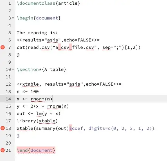
<<results="asis",echo=FALSE>>=
cat(read.csv("a_csv_file.csv", sep=";")[1,2])
@

Or a table:

<<xtable, results="asis">>=
n <- 100
x <- rnorm(n)
y <- 2*x + rnorm(n)
out <- lm(y ~ x)
library(xtable)
xtable(summary(out)$coef, digits=c(0, 2, 2, 1, 2))
@

(Example taken from Karl Broman)

In theory, Knitr supports Python too, but feels weird to use R to execute Python snippets inside LaTeX. So I would advise against Knitr, if you are not using R.

Minimal Example

\documentclass{article}
\begin{document}
The meaning is:
<<results="asis",echo=FALSE>>=
cat(read.csv("a_csv_file.csv", sep=";")[1,2])
@
\section*{A table}
<<xtable, results="asis",echo=FALSE>>=
n <- 100
x <- rnorm(n)
y <- 2*x + rnorm(n)
out <- lm(y ~ x)
library(xtable)
xtable(summary(out)$coef, digits=c(0, 2, 2, 1, 2))
@
\end{document}

The code above is stored as knitr_test.Rnw and a tex file is created using:

R -e 'library(knitr);knit("knitr_test.Rnw")'

The tex file looks like this:

\documentclass{article}
% knitr inserts a lot of stuff in the header, omitted here for simplicity
\begin{document}
The meaning is:
42
\section*{A table}
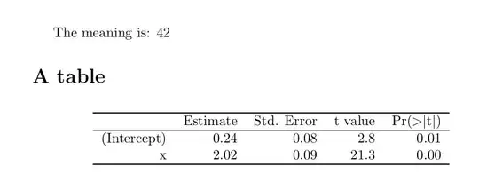
% latex table generated in R 4.3.2 by xtable 1.8-4 package
% Wed Jan 17 17:53:32 2024
\begin{table}[ht]
\centering
\begin{tabular}{rrrrr}
  \hline
 & Estimate & Std. Error & t value & Pr($>$$|$t$|$) \ 
  \hline
(Intercept) & 0.24 & 0.08 & 2.8 & 0.01 \ 
  x & 2.02 & 0.09 & 21.3 & 0.00 \ 
   \hline
\end{tabular}
\end{table}
\end{document}

This is the rendered result:

Overleaf

The online LaTeX Overleaf supports Knitr out of the box. Simply rename your LaTeX file to *.Rtex.

Unfortunately the syntax checking does not seem to support the Knitr syntax:

Downsides

• An additional step during the compilation of the LaTeX file is necessary.
• The code to include a single value is quite long.

More resources

Here is a nice and short tutorial on how to use Knitr with LaTeX.

There is a nice overview for Knitr available in the documentation of overleaf.

This Q&A discusses how to avoid using cat(), which is necessary to hide the output prefix [1].

Answer 3

You are searching the concept of literate programming, that actually is not limited to LaTeX with R trough knitr, but probably has been the most successful proof of concept in last years.

But for general literate programming, not limited to R, nor Python, and not limited to LateX, I suggest Quarto. Quarto can create dynamic content with Python, R, Julia, and Observable to produce a PDF via LaTeX or ConTeXt (and several other formats, but that is off topic here...).

Quarto will use by default the Knitr engine if there any R chunk but Jupyter is the executable code is another language (python, julia, bash, etc.). See here for the detail of the engine selection.

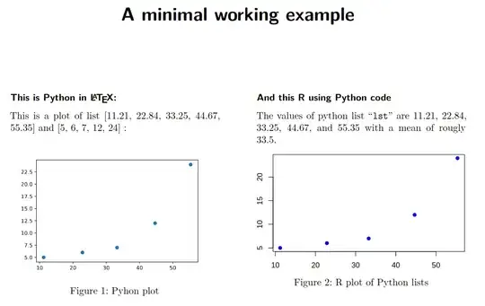
Finally, Knitr supports Python and many other languages, not only "in theory". It is not a mortal sin to execute Python via R, while it work. Moreover, this could have some advantages, since allow run snippets of both languages in the same document and even pass variables from one language to the other, e.g.:

---
title : A minimal working example
format: pdf
classoption: twocolumn 
header-includes: \columnsep1.5cm
---
#| echo: false
library(reticulate)

This is Python in \LaTeX:
#| echo: false
#| results: asis

import matplotlib.pyplot
import pylab
lst = [11.21,22.84,33.25,44.67,55.35] 
lst2 = [5,6,7,12,24] 
print("This is a plot of list") 
print(lst)
print("and") 
print(lst2)
print(":") 


#| echo: false
#| fig-cap: Pyhon plot
matplotlib.pyplot.scatter(lst,lst2)

\newpage
And this R using Python code
The values  of  python list "lst" are
r knitr::combine_words(py$lst) with a mean 
of rougly  r round(mean(py$lst),1).
#| echo: false
#| results: asis
#| fig.cap: R plot of Python lists
#| fig-height: 4
plot(py$lst,py$lst2,ylab="",
xlab="",col="blue",pch=19)

You can add engine: jupyterto the header to avoid the use of knitr (the R code will be only shows but no executed) o r simply remove the last part (from \newpage to the end) to switch automatically to Jupyter that will run python3 without R nor knitr.

But if this workflow bothers you for some reason, there are also LaTeX packages to run Python directly.

Answer 4

My generic comment on analysing and identifying patterns in your (pst) documents still holds.

However, here's a way to work backwards through document-refactoring.

1. Your target documentation

Taking your screenshot your desired target document may look like this in Latex, neglecting all conventions on typesetting numbers, units etc. for demonstration purposes:

\documentclass[10pt,a4paper]{article}
\begin{document}
% ~~~ target documentation ~~~~~~~~~~~
 The growth of wind power \dots US would have changed by 528 % since 2001. \dots increased by 1106 % \dots increased from 15,348 in 2001 to 81,075 in 2021. \dots increased from 597 $m^2$ in 2001 to 6,607 $m^2$ in 2021, \dots .
\end{document}

2. Refactoring placeholders

Next let's try to introduce placeholders, which allows you to:

• write text before simulation results become available
• define a set of useful placeholders for that purpose

The complexity of the placeholders content is up to you, and certainly a matter of context. Assuming your simulation also creates some kind of comparision I'd place-out a bit more complex text than just numbers.

Now, the best tool for this is using \newcommand rather than \def. (You could also assign these things to tables, databases etc., it doesn't matter.) Unfortunately your naming convention then is somewhat restricted. However, it might be a good idea to follow a scheme like:

• < dat >< purpose >< differntiator >
• e.g. datCompA
• or simply datA

\documentclass[10pt,a4paper]{article}
\newcommand\datA[0]{528 % since 2001}
\newcommand\datB[0]{1106 %}
\newcommand\datC[0]{15,348 in 2001}
\newcommand\datD[0]{81,075 in 2021}
\newcommand\datE[0]{597 $m^2$ in 2001}
\newcommand\datF[0]{6,607 $m^2$ in 2021}
\begin{document}
% ~~~ refactoring simulated data (placeholders ~~~
 The growth of wind power \dots US would have changed by \datA{}. \dots increased by \datB{} \dots increased from \datC{} to \datD{}. \dots increased from \datE{} to \datF{}, \dots .
\end{document}

3. Refactoring for simulation data

Ok, it still compiles as intended. So let's move out those \newcommands:

Target Doc:

\documentclass[10pt,a4paper]{article}
% ~~~ refactoring placeholders ~~~
\input{simdat}
\begin{document}
 The growth of wind power \dots US would have changed by \datA{}. \dots increased by \datB{} \dots increased from \datC{} to \datD{}. \dots increased from \datE{} to \datF{}, \dots .
\end{document}

simdat.tex:

\newcommand\datA[0]{528 \% since 2001}
\newcommand\datB[0]{1106 \%}
\newcommand\datC[0]{15,348 in 2001}
\newcommand\datD[0]{81,075 in 2021}
\newcommand\datE[0]{597 $m^2$ in 2001}
\newcommand\datF[0]{6,607 $m^2$ in 2021}

4. Outline of next refactoring steps

Fine. All you now need to do is to generate the content for simdat.tex, e.g. by:

• postprocessing your stored simulation results, using e.g. scripting languages
• creating and storing said content by your simulation program
• etc.

E.g. it should be a no-brainer to go from data here:

528
2001
...

to content there:

\newcommand\datA[0]{528 \% since 2001}
...

5. Conceptual suggestions

For this specific example this procedures seems to be useful:

• prepare your text with required placeholders, best beforehand
• derive required content of placeholders
• create those placeholders from your simulations
• compile the target doc once simulation runs are done.

Answer 5

Generate new Latex commands for results in a Latex

You can create your own Latex commands: one command for each result. The computation pipeline can run a script which creates a Latex header file including the command definitions and the results. This file can then be included in the Latex document.

This is somewhat similar to the solution via text files and \input. Thanks to @Teepeemm for suggesting this variant of the solution in the comments.

Code snippet 1

Add something like this to your computation pipe line and add all values to the dictionary you need in your Latex document:

LATEX_FILE_NAME = 'result_values.tex'
result_values = {}
meaning_of_life = 42
result_values["meaningoflife"] = f"{meaning_of_life:d}"
- A unit can be passed as string as second parameter: the LaTeX package siunitx will be used to display the quantity.
- Use .2f for rounding to two decimals.
gravity_ms2 = 9.80665
result_values["gravity"] = f"{gravity_ms2:.2f}", "m/s^2"
write_result_values(result_values, LATEX_FILE_NAME)

Code snippet 2

This function writes the Latex header:

import re
def format_latex_command(key, value, unit=None):
    # test if key contains invalid characters for a latex command:
    if not re.match(r"^[a-zA-Z]+$", key):
        raise ValueError(f"Invalid key '{key}': not a valid latex command name")
if unit is not None:
    value = f"\\qty{{{value}}}{{{unit}}}"

return f"\\newcommand{{\\{key}}}{{{value}}}"



def write_result_values(result_values, filename):
    """Write the result values to a latex header file creating new Latex command for each value.
Parameters
----------
result_values : dict
    Results to be written to the Latex header file: keys of the dictionary are the names of the
    latex commands the values are either a single value or a tuple containing the value and the
    unit.
filename : str
    The name of the Latex header file to write the result values to.

"""
result_values_flat = [
    (key, *value) if isinstance(value, tuple) else (key, value)
    for key, value in result_values.items()
]
latex_commands = [format_latex_command(*params) for params in result_values_flat]

with open(filename, "w") as f:
    f.write("\n".join(latex_commands) + "\n")

How to use in the Latex document

After running code snippet 1 above a file result_values.tex is created:

\newcommand{\meaningoflife}{42}
\newcommand{\gravity}{\qty{9.81}{m/s^2}}

...one can then use the new Latex commands to add the values to the text:

\documentclass{article}
\usepackage{siunitx}
\include{result_values}
\begin{document}
\section*{Example of including result values}
The gravity constant is \gravity. And the meaning of life is \meaningoflife.
\end{document}

The rendered result looks like this: