How to draw a 3D hexagonal structure with TikZ?

Question

What is the best way in TikZ to draw a hexagonal stucture in 3D? For example, graphite crystals, honeycombs or stable racks made of hexagonal aligned stiffeners.

I already found this nice solution: Drawing hexagons. But this is only for 2D hexagons.

Currently I'm just writing down all nodes separately with (x,y,z) coordinates. But this has the disadvantages of being (a) very annoying, (b) connecting lines don't care about the layers (lines don't go "behind" plane 2 if I connect plane 1 and 3, it's just drawn on top).

What is the best way of realizing a 3D hexagonal structure in TikZ that takes care of the layers and don't needs all coordinates entered by hand but by an algorithm?

You could interpret the “graphite crystal” examples as a 2D drawing that is xslanted and shrunken in y direction. — Qrrbrbirlbel, Apr 07 '13 at 17:31

Gonzalo Medina · Accepted Answer · 2013-04-08T02:19:39.693

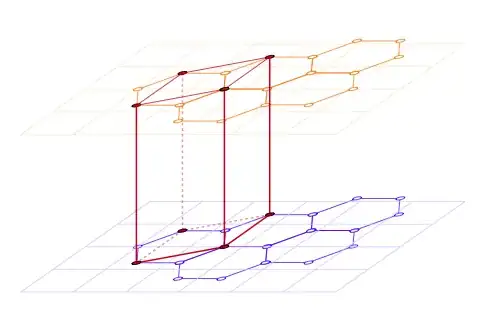
Here's another option, using this time regular polygon from the shapes library; each of the the \hexgrid... commands has two mandatory arguments: the first one, gives a name to the grid and the second one, controls the vertical shifting; the optional argument allows to pass additional options:

\documentclass{article}
\usepackage{tikz}
\usepackage{siunitx}
\usetikzlibrary{arrows,positioning,shapes}

\newcommand\xsla{-1.2}
\newcommand\ysla{0.505}

\newcommand\hexgridv[3][]{%
\begin{scope}[%
  #1
  xscale=-1,
  yshift=#3,
  yslant=\ysla,
  xslant=\xsla,
  every node/.style={anchor=west,regular polygon, regular polygon sides=6,draw,inner sep=0.5cm},
  transform shape
]
\node (A#2) {};
\node (B#2) at ([xshift=-\pgflinewidth,yshift=-\pgflinewidth]A#2.corner 1) {};
\node (C#2) at ([xshift=-\pgflinewidth]B#2.corner 5) {};
\node (D#2) at ([xshift=-\pgflinewidth]A#2.corner 5) {};
\node (E#2) at ([xshift=-\pgflinewidth]D#2.corner 5) {};
\foreach \hex in {A,...,E}
{
  \foreach \corn in {1,...,6}
    \draw[fill=white] (\hex#2.corner \corn) circle (2pt); 
}
\end{scope}
}

\newcommand\hexgridiv[3][]{%
\begin{scope}[%
  #1,
  xscale=-1,
  yshift=#3,
  yslant=\ysla,
  xslant=\xsla,
  every node/.style={anchor=west,regular polygon, regular polygon sides=6,draw,inner sep=0.5cm},
  transform shape
]
\node (A#2) {};
\node (B#2) at (A#2.corner 5) {};
\node[xscale=-1] (C#2) at (B#2.corner 4) {};
\node (D#2) at (C#2.corner 4) {};
\foreach \hex in {A,...,D}
{
  \foreach \corn in {1,...,6}
    \draw[fill=white] (\hex#2.corner \corn) circle (2pt); 
}
\end{scope}
}

\begin{document}

\begin{tikzpicture}[>=latex]
% the three grids
\hexgridv{a}{0}
\hexgridiv[xshift=0.43cm]{b}{-60}
\hexgridv{c}{-160}

% the red lines
\foreach \corn in {2,4}
  \draw[ultra thick,red!80!black] (Aa.corner \corn) -- (Ac.corner \corn);
\draw[ultra thick,red!80!black,opacity=0.4] (Aa.corner 6) -- (Ac.corner 6);
\draw[ultra thick,red!80!black] (Da.corner 4) -- (Dc.corner 4);
\foreach \hexg in {a,c}
  \draw[thick,red!80!black] (A\hexg.corner 2) -- (A\hexg.corner 4) -- (D\hexg.corner 4);
\foreach \hexg/\opac in {a/1,c/0.4}
  \draw[thick,red!80!black,opacity=\opac] (A\hexg.corner 2) -- (A\hexg.corner 6) -- (D\hexg.corner 4);

% the red vertices
\begin{scope}[  yslant=\ysla,xslant=\xsla]
\foreach \hex/\corn in {Aa/2,Aa/4,Aa/6,Ab/3,Ac/2,Ac/4,Da/4,Cb/6,Cb/4,Dc/4} 
  \draw[fill=red!80!black] (\hex.corner \corn) circle (2pt);
\draw[fill=red!80!black,fill opacity=0.4] (Ac.corner 6) circle (2pt);
\draw[fill=red!80!black,fill opacity=0.4] (Cb.corner 2) circle (2pt);
\end{scope}

% The arrows and labels
\draw[help lines] 
  (Aa.corner 2) -- +(2.5,0) coordinate[pos=0.75] (aux1);
\draw[help lines] 
  (Ac.corner 2) -- +(2.5,0) coordinate[pos=0.75] (aux2);
\draw[<->,help lines] 
  (aux1) -- node[pos=0.25,fill=white,font=\footnotesize] {\SI{6.708}{\angstrom}} (aux2);
\draw[help lines] 
  (Ab.corner 2) -- +(1,0) coordinate[pos=0.5] (aux3);
\draw[<->,help lines] 
  (aux3) -- node[fill=white,font=\footnotesize,align=center] {b\\\SI{3.354}{\angstrom}} (aux3|-aux2);
\draw[help lines] 
  (Ac.corner 3) -- +(0,-0.45) coordinate[pos=0.5] (aux4);
\draw[help lines] 
  (Ac.corner 4) -- +(0,-0.4) coordinate[pos=0.5] (aux5);
\draw[<->,help lines] 
  (aux4) -- node[fill=white,font=\footnotesize,align=center,below=1pt] {a\\\SI{1.421}{\angstrom}} (aux5|-aux4);
\end{tikzpicture}

\end{document}

enter image description here

The code admits still improvements, but the main point is that it can be used as a starting point to easily define hexagonal grids. The siunitx package was used to typeset the units (thanks to Svend Tveskæg for the reminder).

One should probably use siunitx (as you know, I assume), if there are a lot of numbers with units. — Svend Tveskæg, Apr 08 '13 at 01:47
\SI{6.708}{\AA} should be \SI{6.708}{\angstrom} (and the same for the other quantities). — Svend Tveskæg, Apr 08 '13 at 02:14
@SvendTveskæg Ah, OK. As you can see, it's the first time I work with units :-) I will edit it. Thank you. — Gonzalo Medina, Apr 08 '13 at 02:15
Thank you very much. :) This is really a great way of doing it. I didn't know that a node can have the shape of a hexagon "automatically". This makes things very comfortable, indeed. :) — Foo Bar, Apr 08 '13 at 08:07

score 10 · Answer 2 · answered Apr 07 '13 at 21:57

I don't know exactly what you want because there are several possibilities to draw 3D hexagonal structure. here an example with tkz-berge

The next code can be adapted:

\documentclass{article}
\usepackage{tkz-berge}
\usetikzlibrary{3d}
\newcommand\pgfmathsinandcos[3]{% 
  \pgfmathsetmacro#1{sin(#3)}% 
  \pgfmathsetmacro#2{cos(#3)}% 
}

\begin{document}

    \pgfmathsetmacro\angFuite{155}
    \pgfmathsetmacro\coeffReduc{1}
    \pgfmathsinandcos\sint\cost{\angFuite}

\begin{tikzpicture}[current plane/.estyle=%
        {cm={1,0,\coeffReduc*\cost,-\coeffReduc*\sint,(0,#1)}}]

\GraphInit[vstyle=Shade]

      \begin{scope}[current plane=0 cm]
         \SetGraphShadeColor{white}{teal}{gray}
         \grEmptyCycle[Math,prefix=a]{6}
     \end{scope}

      \begin{scope}[current plane=6 cm]
         \SetGraphShadeColor{white}{teal}{gray}
         \grEmptyCycle[Math,prefix=b]{6}
     \end{scope}

 \SetGraphShadeColor{white}{teal}{gray}
 \EdgeIdentity*[style={opacity=.3}]{a}{b}{3,4}
 \EdgeInGraphSeq{a}{0}{1}  
 \EdgeInGraphSeq[style={opacity=.3}]{a}{1}{4}
 \Edge(a0)(a5)
 \EdgeInGraphLoop{b}{6}
 \EdgeIdentity*{a}{b}{0,1,2,5}
\end{tikzpicture}
\end{document}

enter image description here

This other example (Author: Andreas Menge) uses another method with tkz-berge and it's easy to adapt

\documentclass[10pt]{article}
\usepackage{tkz-berge}

\newcommand{\myGlobalTransformation}[2]
{
    \pgftransformcm{1}{0}{0.6}{0.2}{\pgfpoint{#1cm}{#2cm}}
}

\begin{document}
\pagestyle{empty}

\begin{tikzpicture}

  \GraphInit[vstyle=Art]
  \begin{scope}
    \myGlobalTransformation{0}{0}
    \grCycle[prefix=a]{5}
  \end{scope}

  \begin{scope}
    \myGlobalTransformation{0}{2}
    \grCycle[prefix=b]{5}
  \end{scope}

  \EdgeIdentity{a}{b}{5}

  \begin{scope}
    \myGlobalTransformation{0}{-2}
    \Vertex{x}
  \end{scope}

  \begin{scope}
    \myGlobalTransformation{0}{4}
    \Vertex{y}
  \end{scope}

  \EdgeFromOneToAll{x}{a}{}{5}
  \EdgeFromOneToAll{y}{b}{}{5}
\end{tikzpicture}

\end{document}

enter image description here

Thanks, also a nice way. :) But I accepted the other answer because it uses just the "plain" TikZ package. — Foo Bar, Apr 08 '13 at 08:11
No problem. It's always interesting for you or other users to know different possibilities to get a result. A possibility is to combine the answers, for example without tkz-berge, you can apply the style curent plan to Gonzalo's method. I will give you another answer with this idea. — Alain Matthes, Apr 08 '13 at 09:21

Alain Matthes · Answer 3 · 2013-04-08T12:23:57.343

Here another answer without tkz-berge. I used a big part of Gonzalo's code but without xslant,yslant but I used a style current plane. This style defines in which plane, I want to draw some objects. You need to define the angle ( angle de fuite french terme in perspective) . If you change this angle sometimes you need to change the opacity for some sides.

Here I use an angle of 175° and then 145°

Update

I added some styles show and hidden. It's more readable.

\documentclass{article}
\usepackage{tikz,fullpage}
\usetikzlibrary{arrows,positioning,shapes}

\newcommand\hexgridv[2][]{%
\begin{scope}[%
  #1,
  every node/.style={anchor=west,regular polygon, regular polygon sides=6,draw,inner sep=0.5cm},transform shape
]
\node (A#2) {};
\node (B#2) at ([xshift=-\pgflinewidth,yshift=-\pgflinewidth]A#2.corner 1) {};
\node (C#2) at ([xshift=-\pgflinewidth]B#2.corner 5) {};
\node (D#2) at ([xshift=-\pgflinewidth]A#2.corner 5) {};
\node (E#2) at ([xshift=-\pgflinewidth]D#2.corner 5) {};
\foreach \hex in {A,...,E}
{
  \foreach \corn in {1,...,6}
    \draw[fill=white] (\hex#2.corner \corn) circle (2pt); 
}
\end{scope}
}

\newcommand\pgfmathsinandcos[3]{% 
  \pgfmathsetmacro#1{sin(#3)}% 
  \pgfmathsetmacro#2{cos(#3)}% 
}

\begin{document}

    \pgfmathsetmacro\angFuite{145}
    \pgfmathsetmacro\coeffReduc{.75}
    \pgfmathsinandcos\sint\cost{\angFuite}

\begin{tikzpicture}[scale=2,
current plane/.estyle={cm={1,0,\coeffReduc*\cost,-\coeffReduc*\sint,(0,#1)}},
show/.style={ultra thick,red!80!black,opacity=1},
hidden/.style={ultra thick,red!80!black,opacity=.4,dashed}]

      \begin{scope}[current plane=0 cm]
        \hexgridv[color=blue]{a}
        \draw[blue!20] (-1,-2) grid (5,2);
     \end{scope}

      \begin{scope}[current plane=3 cm]
        \draw[orange!20] (-1,-2) grid (5,2);
        \hexgridv[color=orange]{c}
     \end{scope}


\begin{scope}[current plane=3 cm]
\foreach \hex/\corn in {Ac/2,Ac/4,Dc/4} 
  \draw[fill=red!80!black] (\hex.corner \corn) circle (2pt);
\draw[fill=red!80!black,fill opacity=0.4] (Ac.corner 6) circle (2pt);
\end{scope}

% the red lines
  \draw[hidden] (Aa.corner 4) -- (Ac.corner 4);
  \draw[hidden] (Da.corner 4) -- (Aa.corner 4) -- (Aa.corner 2) ; 
  \draw[show] (Ac.corner 2) -- (Ac.corner 6) -- (Dc.corner 4) -- (Ac.corner 4) -- (Ac.corner 2);
   \draw[show] (Aa.corner 2) -- (Aa.corner 6) -- (Da.corner 4) 
               (Da.corner 4) -- (Dc.corner 4);
  \foreach \corn in {2,6}
    \draw[show] (Aa.corner \corn) -- (Ac.corner \corn);

% the red vertices
\begin{scope}[current plane=0 cm]
\draw[hidden] (Ac.corner 6) circle (2pt);
\foreach \hex/\corn in {Aa/2,Aa/4,Aa/6,Da/4} 
  \draw[show] (\hex.corner \corn) circle (2pt);
\end{scope}

\end{tikzpicture}
\end{document}

enter image description here

score 5 · Answer 4 · edited Apr 13 '17 at 12:34

By adapting the code from the accepted answer to Drawing hexagons and following Qrrbrbirlbel's advice, you can do this:

enter image description here

\documentclass{article}
\usepackage{tikz}
\usetikzlibrary{positioning}

\newcommand\hexagonalstructure[1]{    \begin{scope}[%
        yshift=#1,
        yslant=0.5,%
        xslant=-1.7,%
    ]
        \foreach \i in {0,...,2} 
        \foreach \j in {0,...,2} {
        \foreach \a in {0,120,-120} \draw (3*\i,2*sin{60}*\j) -- +(\a:1);
        \foreach \a in {0,120,-120} \draw (3*\i+3*cos{60},2*sin{60}*\j+sin{60}) -- +(\a:1);}
    \end{scope}
}

\begin{document}
\begin{tikzpicture}[scale=.5]
    \hexagonalstructure{0}
    \hexagonalstructure{-170}
    \hexagonalstructure{-340}
\end{tikzpicture}
\end{document}

How to draw a 3D hexagonal structure with TikZ?

4 Answers4

Linked