Check out if this MWE with Asymptote does what you need.
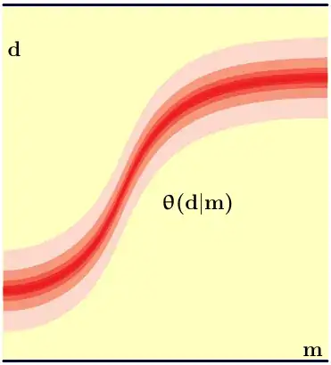
For demonstration in this example it uses three paths (guides)
gtop,gbot and gmid to define functions f(x) for mean
and s(x) for deviation, use the proper definitions
of f(x) and s(x) instead.
Array pen[] clrs defines colors, array real[] dh defines
fractions of the total interval to cover with the corresponding color.
Then for every color the top (gt), bottom (gb) guides
are defined and joined in a region g fo fill with i-th color.
% blurred.tex:
%
\documentclass{article}
\usepackage{textgreek}
\usepackage[inline]{asymptote}
\usepackage{lmodern}
\begin{document}
\begin{figure}
\begin{asy}
size(200);
import graph;

pair[] botP={(0,0.09),(0.252,0.196),(0.383,0.429),(0.479,0.588),
(0.574,0.668),(0.733,0.726),(0.883,0.747),(1,0.747),};

pair[] topP={(0,0.341),(0.252,0.451),(0.383,0.677),(0.479,0.841),
(0.574,0.92),(0.733,0.977),(0.883,0.993),(1,1),};

pair[] midP=0.5*(topP+botP);

guide gtop=graph(topP,operator..);
guide gbot=graph(botP,operator..);
guide gmid=graph(midP,operator..);

real f(real x){
  real t=times(gmid,x)[0];
  return point(gmid,t).y;
};

real s(real x){
  real tt=times(gtop,x)[0];
  real tb=times(gbot,x)[0];
  return point(gtop,tt).y-point(gbot,tb).y;
};

real xmin=0, xmax=1;

pen[] clrs={
  rgb(0.988,0.847,0.796),
  rgb(0.969,0.592,0.502),
  rgb(0.953,0.365,0.29),
  rgb(0.933,0.188,0.165),
  rgb(0.933,0.114,0.137),
};

real[] dh={1,0.5,0.25,0.125,0.0625};

guide gt, gb,g;

for(int i=0;i<clrs.length;++i){
  gt=graph(new real(real x){return f(x)+0.5dh[i]*s(x);},xmin,xmax);
  gb=graph(new real(real x){return f(x)-0.5dh[i]*s(x);},xmin,xmax);
  g=gb--reverse(gt)--cycle;
  fill(g,clrs[i]);
}

real ymax=1.1;
pen axisPen=darkblue+1.3bp;
xaxis(xmin,xmax,axisPen);
xaxis(YEquals(ymax),xmin,xmax,axisPen);

label("\textbf{\straighttheta(d$|$m)}",(0.6,0.5));
label("\textbf{m}",(xmax,0),NW);
label("\textbf{d}",(0,1),SE);

shipout(bbox(Fill(paleyellow)));
\end{asy}
\end{figure}
\end{document}
%
% Process:
%
% pdflatex blurred.tex
% asy blurred-*.asy
% pdflatex blurred.tex


y = f(x)where for eachxin the domain offwe associate a deviations. – juliohm Oct 21 '13 at 13:27\closedcycle(look for section "area plots" in the manual). For every color used, you'd have to provide the point coordinates of both the upper and lower curves, as a single closed path. To automatically blur a single curve sounds more difficult. – iavr Oct 21 '13 at 13:36f(x) +/- wwithwa constant doesn't change its shape. This would mean at every abscissa the confidence interval is the same, which is not the case for the plot shown. – juliohm Oct 21 '13 at 16:53