Block diagram with dsp/TikZ for adaptive feedback cancellation

Question

Hello graphic tex lovers :) I'm trying to draw a diagram in TikZ as close as possible to this one: enter image description here

I'm using the dsp TikZ library and I think my attempt is going in the right direction; however there are a few things I didn't manage to set up properly, as you can see from the MWE

\documentclass{article}
\usepackage{tikz}
\usetikzlibrary{dsp,chains}
\begin{document}

\begin{tikzpicture}

% Blocks and nodes
\node[dspnodeopen,dsp/label=below] (ns) {$v(t)$}; 
\node[dspmultiplier,left=of ns,fill=gray] (mic) {};
\node[dspadder,left=of mic,left=1.5cm] (add) {};
\node[coordinate,left=of add,left=2.35cm]                  (fp1) {};
\node[dspfilter,above=of fp1,above=1.5cm]                     (gain) {$G$};
\node[coordinate,above=of gain,above=1.5cm]                  (fp2) {};
\node[dspnodefull,right=of fp2,right=2.55cm]                  (adnode) {$u(t)$};
\node[dspfilter,right=of gain,right=1.15cm]                     (adfilt) {$\hat{F}$};
\node[dspsquare,right=of fp2,right=4cm]                  (ls) {};
\node[dspfilter,right=of gain,right=4cm]                  (feedback) {F};
\node[dspnodefull,left=of add]                  (afupd1) {};
\node[coordinate,above=of afupd1,above=1cm]                  (afupd2) {};
\node[coordinate,right=of adfilt,above=3.5cm,right=0.5cm]                  (afupd3) {};
% Connections
\draw[dspconn] (ns) -- (mic);
\draw[dspline] (mic) -- node[midway,below=0.09cm] {$y(t)$} (add);
\draw[dspline] (add) -- node[midway,below] {$d[t,\hat{\mathbf{f}}(t)]$} (fp1);
\draw[dspline,dashed] (afupd1) -- (afupd2);
\draw[dspconn,dashed] (afupd2) -- (afupd3);
\draw[dspconn] (fp1) -- (gain);
\draw[dspline] (gain) -- (fp2);
\draw[dspline] (fp2) -- (adnode);
\draw[dspline] (adnode) -- (ls);
\draw[dspconn] (adnode) -- (adfilt);
\draw[dspconn] (adfilt) -- node[midway,right] {$\hat{y}[t |\hat{\mathbf{f}}(t)]$} (add);
\draw[dspconn] (ls) -- (feedback);
\draw[dspconn] (feedback) -- (mic);

 \end{tikzpicture}

 \end{document}

This is what my MWE looks like:

enter image description here

Namely, the things I couldn't properly recreate are:

the microphone and loudspeaker symbols (those gray blocks)
the vertical alignment of the filter blocks
the right positioning of the dashed olique line (it should cut the block with \hat{F} right in the middle)
curved lines to and from the filter block with F
plus and minus signs in the adder.

Is anybody willing to help this poor TikZ user?

Thanks ;)

The answer on Draw simple shortened curved line between two coordinates in TikZ may help you get the curved lines around the filter block. And welcome to TeX.SX! :) — alexwlchan, Mar 21 '14 at 10:38
Thanks Alex! And also thank you for the inclusion of the graphical outcome of my MWE. Regarding the curved lines, I've already tried to use the options out and in, which works with path, but they don't work with the command dspconn defined in dsp... — gbernardi, Mar 21 '14 at 10:50
Hmm. Worked when I did it. Anyway, Gonzalo seems to have you covered. — alexwlchan, Mar 21 '14 at 15:25

score 4 · Accepted Answer · edited Jun 10 '20 at 12:32

One possibility:

\documentclass{article}
\usepackage{tikz}
\usetikzlibrary{dsp,chains,calc,shapes.geometric}
\begin{document}
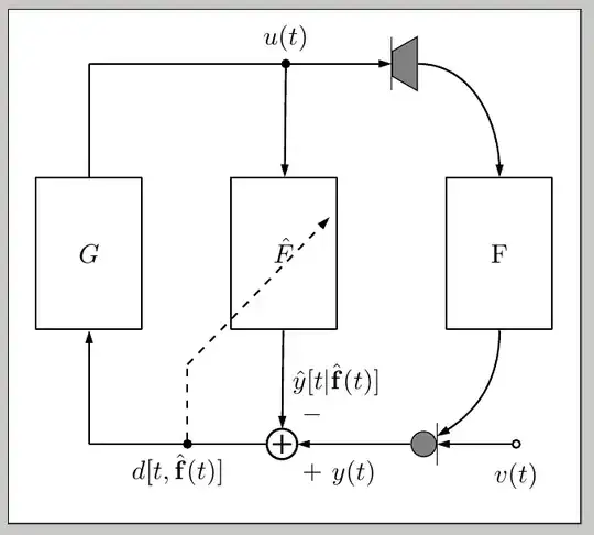
\begin{tikzpicture}
% Blocks and nodes
\node[dspnodeopen,dsp/label=below] 
  (ns) {$v(t)$}; 
\node[left=of ns,fill=gray,circle,draw] 
  (mic) {};
\draw ([yshift=8pt]mic.east) -- ([yshift=-8pt]mic.east);
\node[dspadder,left=of mic,left=1.5cm,label={above right:$-$},label={below right:$+$}] 
  (add) {};
\node[coordinate,left=of add,left=2.35cm]
  (fp1) {};
\node[dspfilter,minimum height=2cm,above=of fp1,above=1.5cm]
  (gain) {$G$};
\node[coordinate,above=of gain,above=1.5cm]
  (fp2) {};
\node[dspnodefull,right=of fp2,right=2.55cm]
  (adnode) {$u(t)$};
\node[dspfilter,minimum height=2cm,right=of gain,right=1.15cm] 
  (adfilt) {$\hat{F}$};
\node[draw,right= 4cm of fp2,fill=gray,trapezium,shape border rotate=90,shape border uses incircle]
  (ls) {};
\draw ([yshift=-10pt]ls.west) -- ([yshift=10pt]ls.west);
\node[dspfilter,minimum height=2cm,right=of gain,right=4cm]
  (feedback) {F};
\node[dspnodefull,left=of add]
  (afupd1) {};
\node[coordinate,above=of afupd1,above=1cm]
  (afupd2) {};
\coordinate (aux) at ([yshift=-4pt]adfilt.center);
% Connections
\draw[dspconn] (ns) -- (mic);
\draw[dspconn] (mic) -- node[midway,below=0.09cm] {$y(t)$} (add);
\draw[dspline] (add) -- node[midway,below] {$d[t,\hat{\mathbf{f}}(t)]$} (fp1);
\draw[dspline,dashed] (afupd1) -- (afupd2);
\draw[dspconn,dashed] (afupd2) -- ( $ (afupd2)!2.7cm!(aux) $ );
\draw[dspconn] (fp1) -- (gain);
\draw[dspline] (gain) -- (fp2);
\draw[dspline] (fp2) -- (adnode);
\draw[dspconn] (adnode) -- (ls);
\draw[dspconn] (adnode) -- (adfilt);
\draw[dspconn] (adfilt) -- node[midway,right] {$\hat{y}[t |\hat{\mathbf{f}}(t)]$} (add);
\draw[dspconn] (ls) to[out=0,in=90] (feedback);
\draw[dspconn] (feedback) to[out=-90,in=30] ([yshift=3pt]mic.east);
\end{tikzpicture}
\end{document}

enter image description here

The answers to specific questions:

Use standard TikZ shapes. The speaker, for example, is simply a rotated trapezium from the shapes.geometric library.
No need for additional tweaks. You can use the standard minimum height key for the dspfilter nodes.
I placed an auxiliary coordinate at adfilt.center (slightly shifted downwards to preven the line from overlapping the "F") and then used the ( $ (<name1>)!<length>!(<name2>) $ ) from the calc library.
You can use to[out=<angle1>,in=<angle2>].
I placed the desired labels to the add node.

In a comment, some problem with cut labels was mentioned when including the figure from an external file. In this case, I'd suggest you to use the standalone class to produce your image as a separate pdf file that then can be easily included in your document using the standard \includegraphics mechanism from graphicx; you can use the border option for standalone to control the padding around your figure, in case it is required:

For example, save the following as, say, MyImage.tex:

\documentclass[tikz,border=10pt]{standalone}
\usetikzlibrary{dsp,chains,calc,shapes.geometric}
\begin{document}
\begin{tikzpicture}
% Blocks and nodes
\node[dspnodeopen,dsp/label=below] 
  (ns) {$v(t)$}; 
\node[left=of ns,fill=gray,circle,draw] 
  (mic) {};
\draw ([yshift=8pt]mic.east) -- ([yshift=-8pt]mic.east);
\node[dspadder,left=of mic,left=1.5cm,label={above right:$-$},label={below right:$+$}] 
  (add) {};
\node[coordinate,left=of add,left=2.35cm]
  (fp1) {};
\node[dspfilter,minimum height=2cm,above=of fp1,above=1.5cm]
  (gain) {$G$};
\node[coordinate,above=of gain,above=1.5cm]
  (fp2) {};
\node[dspnodefull,right=of fp2,right=2.55cm]
  (adnode) {$u(t)$};
\node[dspfilter,minimum height=2cm,right=of gain,right=1.15cm] 
  (adfilt) {$\hat{F}$};
\node[draw,right= 4cm of fp2,fill=gray,trapezium,shape border rotate=90,shape border uses incircle]
  (ls) {};
\draw ([yshift=-10pt]ls.west) -- ([yshift=10pt]ls.west);
\node[dspfilter,minimum height=2cm,right=of gain,right=4cm]
  (feedback) {F};
\node[dspnodefull,left=of add]
  (afupd1) {};
\node[coordinate,above=of afupd1,above=1cm]
  (afupd2) {};
\coordinate (aux) at ([yshift=-4pt]adfilt.center);
% Connections
\draw[dspconn] (ns) -- (mic);
\draw[dspconn] (mic) -- node[midway,below=0.09cm] {$y(t)$} (add);
\draw[dspline] (add) -- node[midway,below] {$d[t,\hat{\mathbf{f}}(t)]$} (fp1);
\draw[dspline,dashed] (afupd1) -- (afupd2);
\draw[dspconn,dashed] (afupd2) -- ( $ (afupd2)!2.7cm!(aux) $ );
\draw[dspconn] (fp1) -- (gain);
\draw[dspline] (gain) -- (fp2);
\draw[dspline] (fp2) -- (adnode);
\draw[dspconn] (adnode) -- (ls);
\draw[dspconn] (adnode) -- (adfilt);
\draw[dspconn] (adfilt) -- node[midway,right] {$\hat{y}[t |\hat{\mathbf{f}}(t)]$} (add);
\draw[dspconn] (ls) to[out=0,in=90] (feedback);
\draw[dspconn] (feedback) to[out=-90,in=30] ([yshift=3pt]mic.east);
\end{tikzpicture}
\end{document}

After processing it through pdflatex you'll get a MyImage.pdf file looking like (gray area around the figure is not part of the resulting pdf):

enter image description here

Then you can use

\usepackage{graphicx}% in preamble
\includegraphics{MyImage}% in document body

in your .tex file to include the image. You can control individual margins with the boder key (refer to the standalone documentation).

Thank you very much for your help Gonzalo! That's (almost) exactly what I was aiming for :)
The second item on the list refers to the fact that, in the original scheme, the three filter blocks are tall rectangles instead of wide rectangle and that's the result I'd like to achieve. Any idea? — gbernardi, Mar 21 '14 at 14:01
@gbernardi: you can play with minimim width and minimum height of the nodes ;) — Claudio Fiandrino, Mar 21 '14 at 15:27
@ClaudioFiandrino: I tried and it now works. I, stupidly, thought you couldn't redefine those properties given that they are defined in the style file. Thanks again guys.
EDIT: an additional small question. I included my figure in a latex file and noticed that some of the labels have been cut. Is that a problem depending on the latex file itself or can I include some additional options to the tikzpicture environment to avoid such cuts? — gbernardi, Mar 21 '14 at 16:20
@gbernardi: Interesting, neither of those keys worked when I tried them. Anyway, I’ve written a second answer which doesn’t use those. :) — alexwlchan, Mar 21 '14 at 16:25
@gbernardi Ah, now I see what you meant in question 2) please see my updated answer. No need for special "tweaks" as in the other answer. Additionally I addressed the problem you mentioned with cut labels. My suggestion (illustrated with a step-by-step example) is to use the standalone class and its border key. — Gonzalo Medina, Mar 21 '14 at 19:23
Thanks for all the suggestions @GonzaloMedina. I tried the solution with the standalone to avoid labels' clipping and it works, but in that way there can be some risk due to improper font scaling.
A solution I found consists in placing some dummy nodes in the "critical areas", where clipping occurs. Not very elegant and figure-dependent for sure, but still working ;) — gbernardi, Mar 24 '14 at 08:27

score 1 · Answer 2 · answered Mar 21 '14 at 16:24

I took Gonzalo’s code, and tweaked it to solve question 2 (the size of the filters).

The dsp library contains a command \dspfilterwidth which sets the width of filter blocks (which is why they seem to play badly with minimum width and minimum height, at least in my testing).

So I started by making that something slightly more amenable, and extending the dspfilter style to get a particular height for the filters:

\renewcommand{\dspfilterwidth}{8mm}

\newcommand{\dspfilterheight}{1.8cm}
\tikzset{dspfilter/.append style = {minimum height=\dspfilterheight}}

Unfortunately, this messes up the spacing of a lot of the blocks, so I went through the node code and tweaked some of it so that the blocks line up, even if you choose different constants yourself.

I also added math mode symbols to the rightmost filter: it should be $F$ instead of plain F if you want it to match the original diagram.

Here’s my tweaked code:

\documentclass{article}
\usepackage{tikz}
\usetikzlibrary{dsp,chains,calc,shapes.geometric}

\begin{document}

\begin{tikzpicture}

\renewcommand{\dspfilterwidth}{8mm}
\newcommand{\dspfilterheight}{1.8cm}

\tikzset{dspfilter/.append style = {minimum height=\dspfilterheight}}

\newcommand{\dspvspace}{1.2cm}

% Blocks and nodes
\node[dspnodeopen, dsp/label=below]
  (ns) {$v(t)$}; 
\node[left=of ns, fill=gray, circle, draw]
  (mic) {};
\draw ([yshift=8pt] mic.east) -- ([yshift=-8pt] mic.east);
\node[dspadder, left=of mic, left=2.35cm, label={above right:$-$}, label={below right:$+$}]
  (add) {};
\node[coordinate, left=of add, left=1.8cm]
  (fp1) {};
\node[dspfilter, above=of fp1, above=\dspvspace]
  (gain) {$G$};
\node[coordinate, above=of gain, above=\dspvspace]
  (fp2) {$fp2$};
\node[dspnodefull, above=of add, above=2*\dspvspace+\dspfilterheight-0.5*\dspoperatordiameter-\dspblocklinewidth]
  (adnode) {$u(t)$};
\node[dspfilter, above=of add, above=\dspvspace-0.5*\dspoperatordiameter] 
  (adfilt) {$\hat{F}$};
\node[draw, above=of mic, above=2*\dspvspace+\dspfilterheight-\dspblocklinewidth-0.4cm, fill=gray, trapezium, shape border rotate=90, shape border uses incircle]
  (ls) {};
\draw ([yshift=-10pt] ls.west) -- ([yshift=10pt] ls.west);
\node[dspfilter, above=of ns, above=\dspvspace]
  (feedback) {$F$};
\node[dspnodefull, left=of add, left=0.8cm]
  (afupd1) {};
\node[coordinate, above=of afupd1, above=\dspvspace]
  (afupd2) {};
\coordinate (aux) at (adfilt.center);

% Connections

\draw[dspconn] (ns) -- (mic);
\draw[dspconn] (mic) -- node[midway,below=0.09cm] {$y(t)$} (add);
\draw[dspline] (add) -- node[midway,below] {$d[t,\hat{\mathbf{f}}(t)]$} (fp1);
\draw[dspline,dashed] (afupd1) -- (afupd2);
\draw[dspconn,dashed] (afupd2) -- ( $ (afupd2)!3cm!(aux) $ );
\draw[dspconn] (fp1) -- (gain);
\draw[dspline] (gain) -- (fp2);
\draw[dspline] (fp2) -- (adnode);
\draw[dspconn] (adnode) -- (ls);
\draw[dspconn] (adnode) -- (adfilt);
\draw[dspconn] (adfilt) -- node[midway,right] {$\hat{y}[t |\hat{\mathbf{f}}(t)]$} (add);
\draw[dspconn] (ls) to[out=0,in=90] (feedback);
\draw[dspconn] (feedback) to[out=-90,in=30] ([yshift=3pt]mic.east);

\end{tikzpicture}

\end{document}

and here’s what it produces:

enter image description here

As I said in one of the previous comments, changing those parameters works for me (at least with the tex file I'm using). In case I need to use it in another tex file where it doesn't work, I'll keep in mind this alternative solution ;) — gbernardi, Mar 21 '14 at 16:42

Block diagram with dsp/TikZ for adaptive feedback cancellation

2 Answers2

The answers to specific questions: