How would you produce the following exact hexagon?

Question

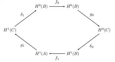
I'm somewhat familiar with the array environment, but I'm not sure what the best approach would be to produce this diagram:

How would I make this, or diagrams similar to this? The slanted arrows and the positioning are what mainly throw me off.

Answer 1

I'd use TikZ to draw that diagram

\documentclass{article}
\usepackage{tikz}
\begin{document}
\begin{tikzpicture}[>=latex]
    \def\radius{2cm} % change to an appropriate value
    \node (h0A) at (60:\radius)   {$H^0(A)$};
    \node (h0C) at (0:\radius)    {$H^0(C)$};
    \node (h1B) at (-60:\radius)  {$H^1(B)$};
    \node (h1A) at (-120:\radius) {$H^1(A)$};
    \node (h1C) at (180:\radius)  {$H^1(C)$};
    \node (h0B) at (120:\radius)  {$H^0(B)$};

    \path[->,font=\small]
        (h0A) edge node[auto] {$g_0$} (h0C)
        (h0C) edge node[auto] {$\delta_0$} (h1B)
        (h1B) edge node[auto] {$f_1$} (h1A)
        (h1A) edge node[auto] {$g_1$} (h1C)
        (h1C) edge node[auto] {$\delta_1$} (h0B)
        (h0B) edge node[auto] {$f_0$} (h0A);
\end{tikzpicture}
\end{document}

First the 6 vertices are defined (as nodes in TikZ-speak) using polar coordinates. They are named (h0A) to (h0B). Then the arrows are drawn using edge paths ((start) edge (finish)) and the descriptions (again nodes) are placed beside them with node[auto] {text}.

A nice introduction to drawing commutative diagrams with TikZ is Commutative Diagrams with TikZ.

Answer 2

Here's a way with Xy-pic

\documentclass[a4paper]{article}
\usepackage[all,cmtip,pdf]{xy}
\usepackage{amsmath}
\begin{document}
\begin{equation}
\begin{gathered}
\xymatrix@C-1em{
& H^0(B) \ar[rr]^{f_0} && H^0(A) \ar[dr]^{g_0} \
H^1(C) \ar[ur]^{\delta_1} &&&& H^0(C) \ar[dl]^{\delta_0} \
& H^1(A) \ar[ul]^{g_1} && H^1(B) \ar[ll]^{f_1}
}
\end{gathered}
\end{equation}
\end{document}

Remember to put the \xymatrix inside a gathered environment if you need an equation number next to it. Otherwise discard the gathered environment.

I've reduced the column distance and doubled the middle arrow across an empty column to keep uniform the arrow lengths.

Update

With tikz-cd:

\documentclass[a4paper]{article}
\usepackage{amsmath}
\usepackage{tikz-cd}
\begin{document}
\begin{equation}
\begin{gathered}
\begin{tikzcd}
  & H^0(B) \arrow[r,"f_0"] &[1em] H^0(A) \arrow[dr,"g_0"] \
H^1(C) \arrow[ur,"\delta_1"] &&& H^0(C) \arrow[dl,"\delta_0"] \
  & H^1(A) \arrow[ul,"g_1"] & H^1(B) \arrow[l,"f_1"]
\end{tikzcd}
\end{gathered}
\end{equation}
\end{document}

Answer 3

Run with xelatex

\documentclass{article}
\usepackage{pst-node}

\begin{document}

\def\R{2.5}
\begin{pspicture}(-3,-3)(3,3)
\psframe*[linecolor=red!10](-3,-3)(3,3)
\psset{nodesep=3pt,arrows=->,shortput=nab}\degrees[6]
\psnode(\R;0){P0}{$H^0(C)$} \psnode(\R;1){P1}{$H^0(B)$}
\psnode(\R;2){P2}{$H^0(B)$} \psnode(\R;3){P3}{$H^1(C)$}
\psnode(\R;4){P4}{$H^1(A)$} \psnode(\R;5){P5}{$H^1(B)$}
\ncline{P0}{P5}^{$\delta_0$}\ncline{P5}{P4}^{$f_1$}
\ncline{P4}{P3}^{$g_1$}     \ncline{P3}{P2}^{$\delta_1$}
\ncline{P2}{P1}^{$f_0$}     \ncline{P1}{P0}^{$g_0$}
\end{pspicture}

\end{document}

Answer 4

I fear I have been beaten...

\documentclass{article}

\usepackage{tikz}
\usetikzlibrary{matrix,arrows}

\begin{document}

\begin{tikzpicture}

% define matrix
\matrix (m) [matrix of nodes, column sep=3em, row sep=3em]
{  & $H^{0}(B)$ & $H^{0}(A)$ &\\
$H^{1}(C)$ &  &  &  $H^{0}(C)$ \\
 & $H^{1}(A)$ & $H^{1}(B)$ & \\};

\path[->, font=\scriptsize]
(m-2-1) edge node[above] {$\delta_{1}$} (m-1-2);

\path[->, font=\scriptsize]
(m-1-2) edge node[above] {$f_{0}$} (m-1-3);

\path[->, font=\scriptsize]
(m-1-3) edge node[above] {$g_{0}$} (m-2-4);

\path[->, font=\scriptsize]
(m-3-3) edge node[below] {$f_{0}$} (m-3-2);

\path[->, font=\scriptsize]
(m-2-4) edge node[below] {$\delta_{0}$} (m-3-3);

\path[->, font=\scriptsize]
(m-3-2) edge node[below] {$g_{1}$} (m-2-1);

\end{tikzpicture}

\end{document}

Answer 5

Another option is to use PSTricks, see below. As always, there's more than way to do this!

See the pst-node documentation for more details and plenty of examples.

\documentclass{article}

\usepackage{pst-node}

\begin{document}

$ \psmatrix[colsep=1.5cm,rowsep=1.5cm]
        &  H^0(B)   & H^0(B)    &     \\
H^1(C)   &           &           & H^0(C)     \\
        &  H^1(A)   & H^1(B)    &     
\endpsmatrix
\psset{nodesep=3pt,arrows=->}
\ncline{2,1}{1,2}\naput{\delta_1}
\ncline{1,2}{1,3}\naput{f_0}
\ncline{1,3}{2,4}\naput{g_0}
\ncline{2,4}{3,3}\naput{\delta_0}
\ncline{3,3}{3,2}\naput{f_1}
\ncline{3,2}{2,1}\naput{g_1}
$

\end{document}