Intersection of a sphere with a paraboloid

Question

I need help in order to draw the intersection of a sphere with a paraboloid. The plotting of these two surfaces by using their equations is too difficult for me, so I used the following code:

\documentclass{article}

   \usepackage{pgfplots}
   \usepackage{tikz}
   \usetikzlibrary{calc}
   \usetikzlibrary{arrows}

\begin{document}

 \begin{tikzpicture}

     \draw node[below] at (0,0,0) {$O$} coordinate (O);

     \draw[->](0,0,0)--(0,3,0);
     \draw node[below left] at (0,3,0) {$z$};

     \draw[->](0,0,0)--(3,0,0);
     \draw node[below left] at (3,0,0) {$y$};

     \draw[->](0,0,0)--(0,0,4.5);
     \draw node[above left] at (0,0,4.5) {$x$};

     \shade[ball color = gray!40, opacity = 0.1] (0,0) circle (2cm);
     \draw[thick,black](0,0) circle (2cm);
     \draw[black](-2,0) arc (180:360:2 and 0.4);
     \draw[densely dotted] (2,0) arc (0:180:2 and 0.4) coordinate (c);
     \fill[fill=black] (0,0) circle (1pt);

     \draw[densely dotted] (-1.475,1.335) arc (170:10:1.5cm and 0.3cm) coordinate[pos=0] (a);

     \draw[black] (-1.475,1.335) arc (-170:-10:1.5cm and 0.3cm) coordinate (b);

     \draw[densely dotted,black] (a) -- (b);

     \draw[densely dotted,black] (c) -- (O);

     \fill[fill=black] (0,1.335) circle (1pt);

 \end{tikzpicture}

\end{document} 

How can I simulate the paraboloid, something like this:

?

Moreover, I would highly appreciate an example of plotting these two surfaces, by knowing their Cartesian/parametric equations, e.g. x^2+y^2+z^2=3, 2*z=x^2+y^2.

Answer 1

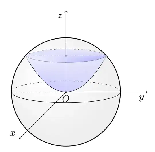
Something like this?

\documentclass{article}

   \usepackage{pgfplots}
   \usepackage{tikz}
   \usetikzlibrary{calc}
   \usetikzlibrary{arrows}

\begin{document}

 \begin{tikzpicture}

     \draw node[below] at (0,0,0) {$O$} coordinate (O);

     \draw[->](0,0,0)--(0,3,0);
     \draw node[below left] at (0,3,0) {$z$};

     \draw[->](0,0,0)--(3,0,0);
     \draw node[below left] at (3,0,0) {$y$};

     \draw[->](0,0,0)--(0,0,4.5);
     \draw node[above left] at (0,0,4.5) {$x$};

     \shade[ball color = gray!40, opacity = 0.1] (0,0) circle (2cm);
     \draw[thick,black](0,0) circle (2cm);
     \draw[black](-2,0) arc (180:360:2 and 0.4);
     \draw[densely dotted] (2,0) arc (0:180:2 and 0.4) coordinate (c);
     \fill[fill=black] (0,0) circle (1pt);

     \draw[densely dotted] (-1.475,1.335) arc (170:10:1.5cm and 0.3cm) coordinate[pos=0] (a);

     \draw[black] (-1.475,1.335) arc (-170:-10:1.5cm and 0.3cm) coordinate (b);

     \draw[densely dotted,black] (a) -- (b);

     \draw[densely dotted,black] (c) -- (O);

     \fill[fill=black] (0,1.335) circle (1pt);

     \draw [variable=\x,samples=50,domain=-1.475:1.475]  plot ({\x}, {0.6*pow(\x,2)});
     \shade[top color=blue!20!white,bottom color=blue!50!white,opacity=0.75,samples=50] (1.475,1.335) -- 
        plot (-{\x}, {min(1.335,0.6*pow(\x,2))})
     -- (-1.475,1.335) arc (-170:-10:1.5cm and 0.3cm) -- cycle;
     \shade[top color=blue!20!white,bottom color=blue!50!white,opacity=0.75]
     (-1.475,1.335) arc (-170:-10:1.5cm and 0.3cm) --
     (-1.475,1.335) arc (170:10:1.5cm and 0.3cm);
 \end{tikzpicture}

\end{document} 

You may also make use of the TikZ library shadings.

\documentclass{article}

   \usepackage{pgfplots}
   \usepackage{tikz}
   \usetikzlibrary{calc}
   \usetikzlibrary{arrows}
   \usetikzlibrary{shadings}

\begin{document}

 \begin{tikzpicture}

     \draw node[below] at (0,0,0) {$O$} coordinate (O);

     \draw[->](0,0,0)--(0,3,0);
     \draw node[below left] at (0,3,0) {$z$};

     \draw[->](0,0,0)--(3,0,0);
     \draw node[below left] at (3,0,0) {$y$};

     \draw[->](0,0,0)--(0,0,4.5);
     \draw node[above left] at (0,0,4.5) {$x$};

     \shade[ball color = gray!40, opacity = 0.1] (0,0) circle (2cm);
     \draw[thick,black](0,0) circle (2cm);
     \draw[black](-2,0) arc (180:360:2 and 0.4);
     \draw[densely dotted] (2,0) arc (0:180:2 and 0.4) coordinate (c);
     \fill[fill=black] (0,0) circle (1pt);

     \draw[densely dotted] (-1.475,1.335) arc (170:10:1.5cm and 0.3cm) coordinate[pos=0] (a);

     \draw[black] (-1.475,1.335) arc (-170:-10:1.5cm and 0.3cm) coordinate (b);

     \draw[densely dotted,black] (a) -- (b);

     \draw[densely dotted,black] (c) -- (O);

     \fill[fill=black] (0,1.335) circle (1pt);

     \draw [variable=\x,samples=50,domain=-1.475:1.475]  plot ({\x}, {0.6*pow(\x,2)});
     \shade[upper right=blue!20!white,lower left=blue!50!white,opacity=0.75,samples=50] (1.475,1.335) -- 
        plot (-{\x}, {min(1.335,0.6*pow(\x,2))})
     -- (-1.475,1.335) arc (-170:-10:1.5cm and 0.3cm) -- cycle;
     \shade[upper left=blue!20!white,lower right=blue!50!white,opacity=0.75]
     (-1.475,1.335) arc (-170:-10:1.5cm and 0.3cm) --
     (-1.475,1.335) arc (170:10:1.5cm and 0.3cm);

     \draw[gray] (0,1.335) -- (0,1.8);
 \end{tikzpicture}

\end{document}

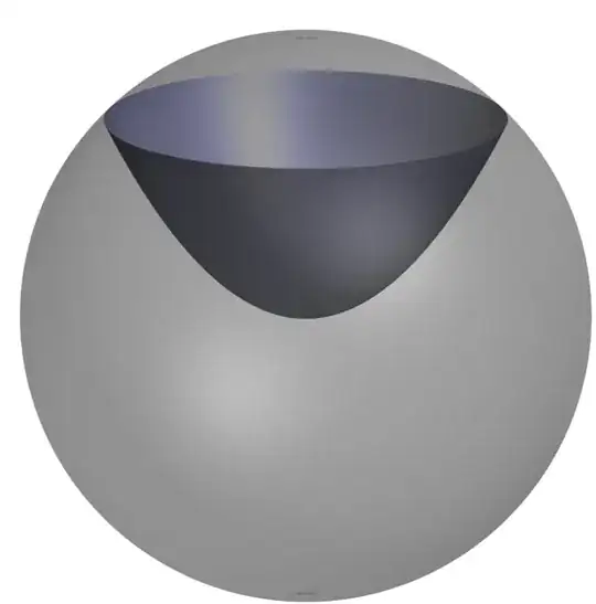
With asymptote you do not have to fake the shadings.

\usepackage{asymptote}
\begin{document}
\begin{asy}
 import graph3;
 import solids;

 size(400); 
 currentprojection=orthographic(4,0,1);
 defaultrender.merge=true;

 defaultpen(0.5mm);

 //Draw the paraboloid: call the radial coordinate r=t.x and the angle phi=t.y
 triple f(pair t) {return ((t.x)*cos(t.y), (t.x)*sin(t.y), (t.x)*(t.x) );
 }

// from https://tex.stackexchange.com/questions/227947/clipping-asymptote-3d-images

 surface s=surface(f,(-1,1),(0,2.32*pi),32,16,
          usplinetype=new splinetype[] {notaknot,notaknot,monotonic},
          vsplinetype=Spline);

 pen p=rgb(0,0,.7); 
 draw(s,rgb(.6,.6,1)+opacity(.7));
 draw(scale3(sqrt(2))*unitsphere,gray+opacity(.3)); 

\end{asy} 
\end{document}