Plot latitude and longitude lines

Question

I am having problems finding how to draw a longitude line like the one show in the figure. I do not want to have a complicate drawing just similar to the one in the picture. I have found some order entries about this issue but are related with more complicated views of a 3d sphere. The problem is hoot draw an arc that passes by the two poles.

Thank you.

This has all been worked out here and here. (At least I think these are the most original posts.) — , Jan 02 '19 at 22:57
Not really, I would like the North and South Poles to be in the upper and downer part of the spare. The plot That I need is much easier that the ones showed in the post. Thanks — Eduardo, Jan 02 '19 at 23:00
Well, these links show how one can draw latitude circles and longitude arcs. What is wrong with taking one of them and drawing these curves using the methods developed there? — , Jan 02 '19 at 23:06
I thought I would be an easier way of doing it. A complicate code for a beginner. — Eduardo, Jan 02 '19 at 23:28
Of course you could just add a cartoon. Or, since you seem not to be interested in distinguishing between hidden visible parts, you could just use tikz-3dplot. — , Jan 02 '19 at 23:30

score 5 · Accepted Answer · 2019-01-03T09:56:34.690

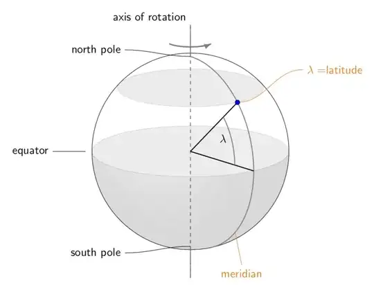
Yes, one can draw such things without caring about whether or nor some element is hidden. Personally like those things produced by these macros, these tricks and many other posts here much better. (If are saying that these should be parts of some packages by now, I would immediately agree, though.) UPDATE: Hide the hidden part of the longitude arc.

\documentclass[tikz,border=3.14mm]{standalone}
\usepackage{tikz-3dplot}
\begin{document}
\tdplotsetmaincoords{105}{0}
\begin{tikzpicture}[tdplot_main_coords,font=\sffamily,line join=bevel]
\pgfmathsetmacro{\R}{3} % radius
\draw[thick,gray,dashed] (0,0,-\R-1) -- (0,0,\R+1);
\begin{scope}
\clip plot[variable=\x,domain=0:180] ({\R*cos(\x)},{\R*sin(\x)},0)
-- plot[variable=\x,domain=180:0,tdplot_screen_coords] ({\R*cos(\x)},{-\R*sin(\x)});
\shade[ball color=gray,opacity=0.2] [tdplot_screen_coords] (0,0) circle (\R);
\end{scope}
\draw[tdplot_screen_coords] (0,0) circle (\R);
% equator
\draw[fill=gray,opacity=0.15] plot[variable=\x,domain=0:360,smooth] ({\R*cos(\x)},{\R*sin(\x)},0);
% upper latitude circle
\pgfmathsetmacro{\Lat}{48}
\draw[fill=gray,opacity=0.15] plot[variable=\x,domain=0:360,smooth] 
({\R*cos(\x)*sin(\Lat)},{\R*sin(\x)*sin(\Lat)},{\R*cos(\Lat)});
% longitude halfcircle with extensions
\pgfmathsetmacro{\Lon}{50}
\pgfmathsetmacro{\thetacrit}{atan(cos(\tdplotmaintheta)/(sin(\tdplotmaintheta)*sin(\Lon)))}
\draw[thick,gray] (0,0,-\R-1) -- (0,0,-\R) 
plot[variable=\x,domain={180+\thetacrit}:0,smooth] 
({\R*cos(\Lon)*sin(\x)},{\R*sin(\Lon)*sin(\x)},{\R*cos(\x)})
-- (0,0,\R+1) node[black,above left] {axis of rotation};
\draw[thick] ({\R*cos(\Lon)*sin(90)},{\R*sin(\Lon)*sin(90)},{\R*cos(90)})
-- (0,0,0) -- ({\R*cos(\Lon)*sin(\Lat)},{\R*sin(\Lon)*sin(\Lat)},{\R*cos(\Lat)})
coordinate (L);
\draw[thick,gray] plot[variable=\x,domain=90:\Lat,smooth] 
({0.7*\R*cos(\Lon)*sin(\x)},{0.7*\R*sin(\Lon)*sin(\x)},{0.7*\R*cos(\x)});
\node [tdplot_screen_coords] at (1,0.4) {$\lambda$};
\draw[orange,tdplot_screen_coords] (L) to[out=0,in=180] ++ (2,1) node[right]{$\lambda=$latitude};
\draw[fill=blue] (L) circle (2pt);
\path (0,0,\R) coordinate (N) (0,0,-\R) coordinate (S) (-\R,0,0) coordinate (W)
({\R*cos(\Lon)*sin(135)},{\R*sin(\Lon)*sin(135)},{\R*cos(135)}) coordinate (M);
\draw[-latex,very thick,gray] plot[variable=\x,domain=150:30,smooth] 
({cos(\x)*sin(\Lat)},{sin(\x)*sin(\Lat)},{\R+0.5});
\draw ([xshift=-2mm]W) -- ++ (-1,0) node[left]{equator}
(N) to[out=180,in=0] ++ (-2,0.2cm) node[left]{north pole}
(S) to[out=180,in=0] ++ (-2,-0.2cm) node[left]{south pole};
\draw[orange,tdplot_screen_coords] (M) -- ++ (0.2,-1) node[below]{meridian};
\end{tikzpicture}
\end{document}

Plot latitude and longitude lines

1 Answers1