Binomial tree converging to a normal distribution (3D)

Question

I try to get the same idea as in Brownian motion 3D normal distribution but with a recombined binomial tree instead of the brownian motion and the corresponding binomial distribution at each node. The idea is to show how the binomial tree converges to a normal distribution. The graph below would be a 2D (not very clean) version. How would it work to get the binomial tree growing in one plane and see the binomial distribution converging to a normal distribution ?

In Binomial distribution we get the binom function

declare function={binom(\k,\n,\p)=\n!/(\k!*(\n-\k)!)*\p^\k*(1-\p)^(\n-\k);}

From recombining-binomial-tree we get the idea of recursive binomial tree. However I don't manage to present even a MWE.

score 4 · Accepted Answer · 2019-01-26T13:50:10.957

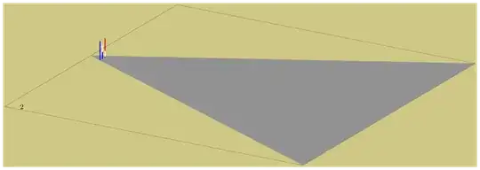
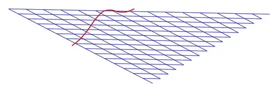
Started from @marmot answer but I don't well understand the coordinates and the shift of -0.5 I needed to do on x coordinate.

\documentclass[tikz,border=3.14mm]{standalone}
\usepackage{tikz-3dplot}
\usetikzlibrary{3d}
\usetikzlibrary{fpu}

\usepackage{xintexpr}
% 8 digits precision is enough
\xintDigits := 8;
% I don't like the order of variables but I picked it up from OP
\xintdeffloatfunc binom(k, n, p) := binomial(n, k)*p^k*(1-p)^(n-k);

\begin{document}

\tdplotsetmaincoords{110}{-30}

\begin{tikzpicture}[binom tree/.style={insert path={%
  foreach \X in {1,...,#1}
 {foreach \Y in {1,...,\X} {(\X,\Y-\X/2) -- (\X+1,\Y+1/2-\X/2)
 (\X,\Y-\X/2) -- (\X+1,\Y-1/2-\X/2)} }}},tdplot_main_coords]

 \begin{scope}[canvas is xy plane at z=0,scale=0.5]

  \draw[blue,binom tree=15];

 \end{scope}

 \tdplotsetrotatedcoords{0}{0}{0}

 \begin{scope}[tdplot_rotated_coords]

  \xintFor* #1 in {\xintSeq{2}{16}}:
  {
  \begin{scope}[canvas is yz plane at x=#1/2, scale=0.5]

   \draw[red,thick] plot[smooth] coordinates {\xintthecoords
     \xintfloatexpr seq((x-#1/2+0.5,8*binom(x, #1, 0.5)), x=0..#1)\relax};

  \end{scope}
  }

 \end{scope}
\end{tikzpicture}
\end{document}

I understand better the coordinates. I think using rescaled bar plots taking into account the "ecart-type" is closer to original question. (But I keep the 3D design from marmot's answer).

\documentclass[tikz,border=3.14mm]{standalone}
\usepackage{tikz-3dplot}
\usetikzlibrary{3d}
\usetikzlibrary{fpu}

\usepackage{xintexpr}
% 8 digits precision is enough
\xintDigits := 8;
% I don't like the order of variables but I picked it up from OP
\xintdeffloatfunc binom(k, n, p) := binomial(n, k)*p^k*(1-p)^(n-k);

\begin{document}

\tdplotsetmaincoords{110}{-30}

\begin{tikzpicture}[binom tree/.style={insert path={%
  foreach \X in {1,...,#1}
 {foreach \Y in {1,...,\X} {(\X,\Y-\X/2) -- (\X+1,\Y+1/2-\X/2)
 (\X,\Y-\X/2) -- (\X+1,\Y-1/2-\X/2)} }}},tdplot_main_coords]

 \begin{scope}[canvas is xy plane at z=0]

  \draw[blue,binom tree=48];

 \end{scope}

 \tdplotsetrotatedcoords{0}{0}{0}

 \begin{scope}[tdplot_rotated_coords]

  \xintFor* #1 in {\xintSeq{0}{48}}:
  {
  \begin{scope}[canvas is yz plane at x=#1+1]
  % ybar means in z direction here, as horizontal coordinate is y
   \draw[red,thick] plot[ybar] coordinates {\xintthecoords
     \xintfloatexpr subs(
           seq((y-#1/2+0.5,A*binom(y, #1, 0.5)), y=0..#1)
          ,A=sqrt(#1))\relax};

  \end{scope}
  }

 \end{scope}
\end{tikzpicture}
\end{document}

Here is with

\begin{tikzpicture}[scale=0.5,binom tree/.style={insert path={%
  foreach \X in {1,...,#1}
 {foreach \Y in {1,...,\X} {(\X,\Y-\X/2) -- (\X+1,\Y+1/2-\X/2)
 (\X,\Y-\X/2) -- (\X+1,\Y-1/2-\X/2)} }}},tdplot_main_coords]

 \begin{scope}[canvas is xy plane at z=0]

  \draw[blue,binom tree=96];

 \end{scope}

 \tdplotsetrotatedcoords{0}{0}{0}

 \begin{scope}[tdplot_rotated_coords]

  \xintFor* #1 in {\xintSeq[6]{0}{96}}:
  {
  \begin{scope}[canvas is yz plane at x=#1+1]
  % ybar means in z direction here, as horizontal coordinate is y
   \fill[red,thick] plot[ybar] coordinates {\xintthecoords
     \xintfloatexpr subs(
           seq((y-#1/2+0.5,A*binom(y, #1, 0.5)), y=0..#1)
          ,A=4*sqrt(#1))\relax};

  \end{scope}
  }

 \end{scope}
\end{tikzpicture}

Most (more then 3/4th) of the time goes into the blue canvas.

Here is with p=0.25.

 \begin{scope}[tdplot_rotated_coords]

  \xintFor* #1 in {\xintSeq[6]{0}{96}}:
  {
  \begin{scope}[canvas is yz plane at x=#1+1]
  % ybar means in z direction here, as horizontal coordinate is y
   \fill[red,thick] plot[ybar] coordinates {\xintthecoords
     \xintfloatexpr subs(
           seq((y-#1/2+0.5,A*binom(y, #1, 0.25)), y=0..#1)
          ,A=4*sqrt(#1))\relax};

  \end{scope}
  }

 \end{scope}

Full code and animation (p=0.25)

\documentclass[tikz,border=3.14mm]{standalone}
\usepackage{tikz-3dplot}
\usetikzlibrary{3d}
\usetikzlibrary{fpu}

\usepackage{xintexpr}
% 8 digits precision is enough
\xintDigits := 8;
% I don't like the order of variables but I picked it up from OP
\xintdeffloatfunc binom(k, n, p) := binomial(n, k)*p^k*(1-p)^(n-k);

\begin{document}

\tdplotsetmaincoords{110}{-30}

  \xintFor* #1 in {\xintSeq[3]{2}{50}}:
  {
\begin{tikzpicture}[scale=0.5,binom tree/.style={insert path={%
  foreach \X in {1,...,#1}
 {foreach \Y in {1,...,\X} {(\X,\Y-\X/2) -- (\X+1,\Y+1/2-\X/2)
 (\X,\Y-\X/2) -- (\X+1,\Y-1/2-\X/2)} }}},tdplot_main_coords]

% \xintifForLast {
 \begin{scope}[canvas is xy plane at z=0]

  \draw[very thin] (1,-25.5)--(51,-25.5) -- (51,25.5)-- (1, 25.5) -- cycle;
  %\draw[blue, very thick] (0,0)--(33,-16.5) -- (33,16.5)-- cycle;
  % \draw[blue,binom tree=32];
  % \draw[blue,binom tree=96];
  \draw[blue, binom tree=#1];

  \draw (#1+1, 25.5) node [right, scale=2] {\smash{\rlap{$#1$}}};
 \end{scope}
% }{}

 \tdplotsetrotatedcoords{0}{0}{0}

 \begin{scope}[tdplot_rotated_coords]

  \begin{scope}[canvas is yz plane at x=#1+1]
  % ybar means in z direction here, as horizontal coordinate is y
   \fill[red,thick] plot[ybar] coordinates {\xintthecoords
     \xintfloatexpr subs(
           seq((y-#1/2+0.5,A*binom(y, #1, 0.25)), y=0..#1)
          ,A=4*sqrt(#1))\relax};

  \end{scope}

 \end{scope}
\end{tikzpicture}
  }

\end{document}

Do pdflatex on this and then

convert -verbose -delay 75 -loop 0 -density 100 binomialplotV.pdf binomialplotV.gif

With p=0.15, 0.5, 0.85. Notice how central case is more spread-out which is normal as variance is larger for it.

(it shows better when zooming)

The 4 in rescaling by A=4*sqrt(#1) was chosen to be big enough so that one sees something and not provoque collisions. The #1 is taken along an arithmetic progression of parameter 6. So at very right we have n=96. — , Jan 26 '19 at 11:23
What a powerful graph ! thank you @jfbu. I am going to try to animate the tree with so that i can break step by step, n by n (or every 5 n), the progression to a normal distribution. — JeT, Jan 26 '19 at 11:28
Setting-up and drawing the blue canvas takes much time, I wonder if you can compute it once and store it for reuse for your animation. I don't know much TikZ. But surely you can move the \xintFor loop to outside to do 16 pictures instead of one. I will it do it for fun with no canvas and make an animated gif, but I think nowadays with TikZ 3.1 you can produce svg output. — , Jan 26 '19 at 11:41
(depending on zoom level in web browser, the animation may appear to have some holes in blue stuff) — , Jan 26 '19 at 12:16

score 2 · Answer 2 · 2019-01-26T03:49:24.387

This is a quickly written proposal, in which I approximate the binomial distribution by a Gaussian.

\documentclass[tikz,border=3.14mm]{standalone}
\usepackage{tikz-3dplot}
\usetikzlibrary{3d}
\begin{document}
\tdplotsetmaincoords{110}{-30}
\begin{tikzpicture}[binom tree/.style={insert path={%
foreach \X in {1,...,#1}
 { foreach \Y in {1,...,\X} {(\X,\Y-\X/2) -- (\X+1,\Y+1/2-\X/2)
 (\X,\Y-\X/2) -- (\X+1,\Y-1/2-\X/2)} }}},tdplot_main_coords]
 \begin{scope}[canvas is xy plane at z=0,scale=0.5]
  \draw[blue,binom tree=15];
 \end{scope} 
 \tdplotsetrotatedcoords{0}{0}{0}
 \begin{scope}[tdplot_rotated_coords,declare function={gauss(\x,\y,\z)=1/(\y*sqrt(2*pi))*exp(-((\x-\z)^2)/(2*\y^2));}]
  \begin{scope}[canvas is yz plane at x=4,scale=0.5]
   \draw[red,thick] plot[variable=\x,domain=-4:4,samples=51,smooth] (\x+0.5,{6*gauss(\x,1,0)});
  \end{scope}
  \begin{scope}[canvas is yz plane at x=8,scale=0.5]
   \draw[red,thick] plot[variable=\x,domain=-8:8,samples=51,smooth] (\x+0.5,{6*gauss(\x,2,0)});
  \end{scope}
 \end{scope}
\end{tikzpicture}
\end{document}

With the fpu library you can plot some binomial distribution, but unfortunately it does not get you very far.

\documentclass[tikz,border=3.14mm]{standalone}
\usepackage{tikz-3dplot}
\usetikzlibrary{3d}
\usetikzlibrary{fpu} 
\begin{document}
\tdplotsetmaincoords{110}{-30}
\begin{tikzpicture}[binom tree/.style={insert path={%
foreach \X in {1,...,#1}
 { foreach \Y in {1,...,\X} {(\X,\Y-\X/2) -- (\X+1,\Y+1/2-\X/2)
 (\X,\Y-\X/2) -- (\X+1,\Y-1/2-\X/2)} }}},tdplot_main_coords]
 \begin{scope}[canvas is xy plane at z=0,scale=0.5]
  \draw[blue,binom tree=15];
 \end{scope} 
 \tdplotsetrotatedcoords{0}{0}{0}
 \begin{scope}[tdplot_rotated_coords,declare
 function={gauss(\x,\y,\z)=1/(\y*sqrt(2*pi))*exp(-((\x-\z)^2)/(2*\y^2));},
 declare function={binom(\k,\n,\p)=\n!/(\k!*(\n-\k)!)*\p^\k*(1-\p)^(\n-\k);}]
  \begin{scope}[canvas is yz plane at x=4,scale=0.5]
   \pgfkeys{/pgf/fpu,/pgf/fpu/output format=fixed} 
   \pgfmathsetmacro{\Z}{4*binom(0,8,0.5)}
   \xdef\lstX{(-3.5,\Z)}
   \foreach \X [count=\Y] in {1,...,8}
   {
   \pgfmathsetmacro{\Z}{4*binom(\X,8,0.5)}
   \xdef\lstX{\lstX (\X-3.5,\Z)}
   }
   \draw[red,thick] plot[smooth] coordinates {\lstX};
  \end{scope}
  \begin{scope}[canvas is yz plane at x=6,scale=0.5]
%    \pgfmathsetmacro{\Z}{binom(1,12,0.5)}
%    \xdef\lstX{(-6,\Z)}
%    \foreach \X [count=\Y] in {1,...,12}
%    {
%    \pgfmathsetmacro{\Z}{binom(\X,12,0.5)}
%    \typeout{\Z}
%    \xdef\lstX{\lstX (\X-6,\Z)}
%    }
%    \draw[red,thick] plot[smooth] coordinates {\lstX};
  \end{scope}
 \end{scope}
\end{tikzpicture}
\end{document}

One can most likely solve the problem by employing the gamma function. Yet I am not sure if this will be distinguishable from the Gaussian.

Binomial tree converging to a normal distribution (3D)

2 Answers2