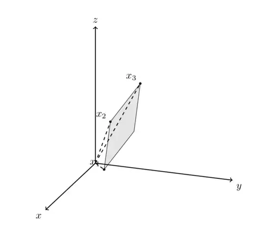
This answer is conceptually the same as the answer to your previous question. Using calc, you can add and subtract vectors. So one way to draw the plane is to say
\draw[fill=gray,fill opacity=0.2] (x_1) -- (x_2) -- (x_3) -- ($(x_3)+(x_1)-(x_2)$) -- cycle;
Full MWE (with \tdplotsetmaincoords{70}{110} added to make the code run through and some simplifications):
\documentclass{article}
\usepackage[margin=1in]{geometry}
\usepackage{tikz, tikz-3dplot}
\usepackage{amsmath}
\begin{document}
\tdplotsetmaincoords{70}{110}
\begin{tikzpicture}[scale=0.5, tdplot_main_coords, axis/.style={->,black,thick},
vector/.style={-stealth,black,very thick},
vector guide/.style={dashed,black,thick}]
    %standard tikz coordinate definition using x, y, z coords
    \path  (0,0,0) coordinate (origin)
     (1,1,0) coordinate (x_1)
     (-3,0,2) coordinate  (x_2)
     (2,4,7) coordinate  (x_3);
    \draw[fill=gray,fill opacity=0.2] (x_1) -- (x_2) -- (x_3)
     -- ($(x_3)+(x_1)-(x_2)$) -- cycle;
    %draw axes
    \draw[axis] (0,0,0) -- (10,0,0) node[anchor=north east]{$x$};
    \draw[axis] (0,0,0) -- (0,10,0) node[anchor=north west]{$y$};
    \draw[axis] (0,0,0) -- (0,0,10) node[anchor=south]{$z$};
    % Draw two points
    \draw[fill=black]
     foreach \X in {1,2,3}
    { (x_\X) circle[radius=2pt] node[anchor=south east]{$x_\X$}};
    %draw guide lines to components
    \foreach \X in {1,2,3}
    {\draw[vector guide] (origin) -- (x_\X);}
\end{tikzpicture}
\end{document}
ADDENDUM: Just for fun: an attempt to let TikZ decide whether the plane is on the foreground or background.
\documentclass[tikz,border=3mm]{standalone}
\usepackage{tikz-3dplot}
\usepackage{amsmath}
\usetikzlibrary{backgrounds}
\makeatletter
\def\RawCoord(#1){\csname tikz@dcl@coord@#1\endcsname}%
\def\scalprod#1=#2.#3;{%
\edef\coordA{\RawCoord#2}%
\edef\coordB{\RawCoord#3}%
\pgfmathsetmacro\pgfutil@tmpa{scalarproduct({\coordA},{\coordB})}
\edef#1{\pgfutil@tmpa}}%
\makeatother
\newcommand{\spaux}[6]{(#1)*(#4)+(#2)*(#5)+(#3)*(#6)}
\pgfmathdeclarefunction{scalarproduct}{2}{% scalar product of two 3-vectors
  \begingroup%
  \pgfmathparse{\spaux#1#2}%
  \pgfmathsmuggle\pgfmathresult\endgroup}
% projections
\pgfmathdeclarefunction{xcomp3}{3}{% x component of a 3-vector
\begingroup%
  \pgfmathparse{#1}%
  \pgfmathsmuggle\pgfmathresult\endgroup}
\pgfmathdeclarefunction{ycomp3}{3}{% y component of a 3-vector
\begingroup%
  \pgfmathparse{#2}%
  \pgfmathsmuggle\pgfmathresult\endgroup}
\pgfmathdeclarefunction{zcomp3}{3}{% z component of a 3-vector
\begingroup%
  \pgfmathparse{#3}%
  \pgfmathsmuggle\pgfmathresult\endgroup}
% allows us to do linear combinations
\def\lincomb#1=#2*#3+#4*#5;{%
\path[overlay] let \p1=#3,\p2=#5 in
({(#2)*(xcomp3\coord1)+(#4)*(xcomp3\coord2)},%
 {(#2)*(ycomp3\coord1)+(#4)*(ycomp3\coord2)},%
 {(#2)*(zcomp3\coord1)+(#4)*(zcomp3\coord2)}) coordinate #1;}
% vector product
\def\vecprod#1=#2x#3;{%
\path[overlay] let \p1=#2,\p2=#3 in
 ({vpx({\coord1},{\coord2})},%
 {vpy({\coord1},{\coord2})},%
 {vpz({\coord1},{\coord2})}) coordinate #1;}
% vector product auxiliary functions
\newcommand{\vpauxx}[6]{(#2)*(#6)-(#3)*(#5)}
\newcommand{\vpauxy}[6]{(#4)*(#3)-(#1)*(#6)}
\newcommand{\vpauxz}[6]{(#1)*(#5)-(#2)*(#4)}
% vector product pgf functions
\pgfmathdeclarefunction{vpx}{2}{% x component of vector product
  \begingroup%
  \pgfmathparse{\vpauxx#1#2}%
  \pgfmathsmuggle\pgfmathresult\endgroup}
\pgfmathdeclarefunction{vpy}{2}{% y component of vector product
  \begingroup%
  \pgfmathparse{\vpauxy#1#2}%
  \pgfmathsmuggle\pgfmathresult\endgroup}
\pgfmathdeclarefunction{vpz}{2}{% z component of vector product
  \begingroup%
  \pgfmathparse{\vpauxz#1#2}%
  \pgfmathsmuggle\pgfmathresult\endgroup}

\begin{document}
\foreach \Angle in {0,10,...,350}
{\tdplotsetmaincoords{70}{\Angle}
\begin{tikzpicture}[scale=0.5, tdplot_main_coords, axis/.style={->,black,thick},
vector/.style={-stealth,black,very thick},
vector guide/.style={dashed,black,thick}]
    \path[use as bounding box,tdplot_screen_coords] (-12,-5) rectangle (12,10);
    %standard tikz coordinate definition using x, y, z coords
    \path  (0,0,0) coordinate (origin)
     (1,1,0) coordinate (x_1)
     (-3,0,2) coordinate  (x_2)
     (2,4,7) coordinate  (x_3);
    %draw axes
    \draw[axis] (0,0,0) -- (10,0,0) node[anchor=north east]{$x$};
    \draw[axis] (0,0,0) -- (0,10,0) node[anchor=north west]{$y$};
    %draw guide lines to components
    \foreach \X in {1,2,3}
    {\draw[vector guide] (origin) -- (x_\X);
    \path (origin) --
    (x_\X) node[circle,inner sep=1pt]{} node[pos=1+0.75/(\X*\X)]{$x_\X$};}
    % define differences of points on the plane
    \lincomb(d1)=1*(x_1)+(-1)*(x_2);
    \lincomb(d2)=1*(x_2)+(-1)*(x_3);
    % normal on plane
    \vecprod(nA)=(d1)x(d2);
    \edef\coordA{\RawCoord(nA)}
    \pgfmathsetmacro\myz{-1*zcomp3(\coordA)}
    \scalprod\myf=(nA).(x_1);
    \draw[axis] (0,0,{\myf/\myz}) -- (0,0,10) node[anchor=south]{$z$};
    % normal of screen
    \path[overlay] ({sin(\tdplotmaintheta)*sin(\tdplotmainphi)},
       {-1*sin(\tdplotmaintheta)*cos(\tdplotmainphi)},
       {cos(\tdplotmaintheta)}) coordinate (n);
    %
    \scalprod\myproj=(nA).(n);
    \pgfmathtruncatemacro{\itest}{sign(\myproj)}
    \ifnum\itest=-1
     \begin{scope}[on background layer]
      \draw[thick] (0,0,0) -- (0,0,{\myf/\myz});
      \draw[fill=gray,fill opacity=0.8] (x_1) -- (x_2) -- (x_3)
       -- ($(x_3)+(x_1)-(x_2)$) -- cycle;
     \end{scope}
    \else
     \draw[thick] (0,0,0) -- (0,0,{\myf/\myz});
     \draw[fill=gray,fill opacity=0.8] (x_1) -- (x_2) -- (x_3)
       -- ($(x_3)+(x_1)-(x_2)$) -- cycle;
    \fi
\end{tikzpicture}}
\end{document}


\coordinate (<name>) at (<coordinate>);and\path (<coordinate>) coordinate (<name>);are sometimes said to be equivalent, but in reality they are not (as of now). If you want to make use of the recent undocumented addition to TikZ that allows you to retrieve 3d coordinates (see e.g. here for an application), you will need the second syntax, which is why I was using it here. – Sep 02 '19 at 21:06