Plot matrix from input data

Question

I have a matrix, M, exported from Matlab to a .dat file. I want to import this into tikz and plot a density plot for the real and imaginary parts of M separately. The x-axis being the column index, y-axis the rows and the z being the value stored in element [M]_{i,j}.

This question was asked and got a reply to in this post. However, the solution required specific manipulation of the data and given that it was asked almost 4 years ago, I'm wondering whether there is an alternative approach.

The data matrix looks like this:

1.083+0.329i    0.329+-0.373i   0-0.139i            -0.139-0.896i
0.329-0.683i    -0.683-0.379i   0.139+0i            4.494e-12+0.215i
0.329-0.683i    -0.683-0.379i   0.139-4.494e-12i    0+0.215i
-0.373-0.379i   -0.379+0.282i   0.896-0.215i        -0.215+0i

Any help is appreciated.

Answer 1

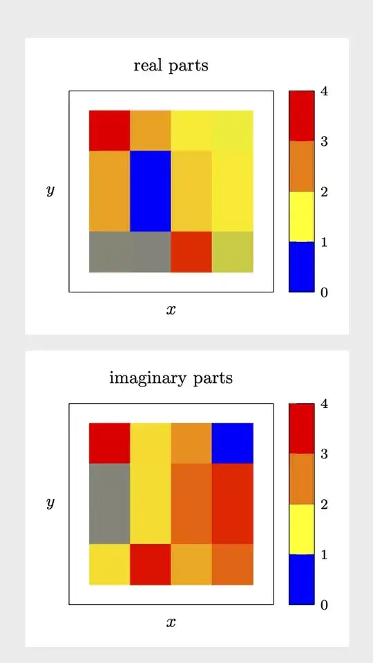
This is some code that reads your table and allows you to produce a matrix plot for the real and imaginary parts. The extraction of the real and imaginary parts uses xstring. For the real part, we just replace i by *0, and parse the result. For the imaginary part, we replace i by *1 and subtract the real part. Seems to work fine.

\documentclass[border=3mm,tikz]{standalone}
\usepackage{pgfplots}
\usetikzlibrary{pgfplots.colormaps}
\pgfplotsset{compat=1.16}
\usepackage{pgfplotstable}
\usepackage{filecontents}
\usepackage{xstring}

\begin{filecontents*}{complexentries.dat}
1.083+0.329i    0.329+-0.373i   0-0.139i            -0.139-0.896i
0.329-0.683i    -0.683-0.379i   0.139+0i            4.494e-12+0.215i
0.329-0.683i    -0.683-0.379i   0.139-4.494e-12i    0+0.215i
-0.373-0.379i   -0.379+0.282i   0.896-0.215i        -0.215+0i
\end{filecontents*}
\def\pgfmathsetmacroFPU#1#2{\begingroup%
\pgfkeys{/pgf/fpu,/pgf/fpu/output format=fixed}%
\pgfmathsetmacro{#1}{#2}%
\pgfmathsmuggle#1\endgroup}%
\newcommand\ExtractRealAndImaginary[1]{%
\StrSubstitute{#1}{i}{*0}[\mytemp]%
\pgfmathsetmacroFPU{\myreal}{\mytemp}%
\StrSubstitute{#1}{i}{*1}[\mytemp]%
\pgfmathsetmacroFPU{\myim}{\mytemp-\myreal}}


\def\ipExtractRealAndImaginary#1+#2i{\def\myreal{#1}\def\myim{#2}}
\def\imExtractRealAndImaginary#1-#2i{\def\myreal{#1}\def\myim{-#2}}
\newcommand*{\ReadOutElement}[4]{%
    \pgfplotstablegetelem{#2}{[index]#3}\of{#1}%
    \let#4\pgfplotsretval
}
\begin{document}
\pgfplotstableread[header=false]{complexentries.dat}\datatable
%\pgfplotstabletypeset\datatable

%\end{document}
\pgfplotstablegetrowsof{\datatable}
\pgfmathtruncatemacro{\numrows}{\pgfplotsretval}
\pgfplotstablegetcolsof{\datatable}
\pgfmathtruncatemacro{\numcols}{\pgfplotsretval}
\foreach \nY in {1,...,\numrows}
{\pgfmathtruncatemacro{\newY}{\numrows-\nY}
\foreach \nX in {1,...,\numcols}
{
\ReadOutElement{\datatable}{\the\numexpr\nY-1}{\the\numexpr\nX-1}{\Current}%
%\typeout{===========}
\edef\temp{\noexpand\ExtractRealAndImaginary{\Current}}
\temp
%\typeout{Re(\Current)=\myreal,Im(\Current)=\myim}
%\edef\myentry{\myim}%
\pgfmathtruncatemacro{\nZ}{\nX+\nY}%
\ifnum\nZ=2
\xdef\LstX{\the\numexpr\nX-1}%
\xdef\LstY{\the\numexpr\nY-1}%
\xdef\LstRe{\myreal}%
\xdef\LstIm{\myim}%
\else
\xdef\LstX{\LstX,\the\numexpr\nX-1}%
\xdef\LstY{\LstY,\the\numexpr\nY-1}%
\xdef\LstRe{\LstRe,\myreal}%
\xdef\LstIm{\LstIm,\myim}%
\fi
}
}
\edef\temp{\noexpand\pgfplotstableset{
 create on use/x/.style={create col/set list={\LstX}},
 create on use/y/.style={create col/set list={\LstY}},
 create on use/real/.style={create col/set list={\LstRe}},
 create on use/im/.style={create col/set list={\LstIm}},
}}
\temp
\pgfmathtruncatemacro{\strangenum}{\numrows*\numcols}
\pgfplotstablenew[columns={x,y,real,im}]{\strangenum}\strangetable

%\pgfplotstabletypeset\strangetable

\begin{tikzpicture}
\begin{axis}[%
    small,title=real parts,
    tick align=outside,
    minor tick num=4,
    %
    xlabel=$x$,
    xlabel near ticks,
    xmin=-1, xmax=4,
    xtick=\empty,
    %
    ylabel=$y$,
    ylabel style={rotate=-90},
    ymin=-1, ymax=4,     
    ytick=\empty,
%     point meta min=0,
%     point meta max=32,
    point meta=explicit,
    %
    %colorbar sampled,
    colorbar as palette,
    colorbar style={samples=3},
    %colormap name=WhiteRedBlack,
    scale mode=scale uniformly,
]
 \addplot [
        matrix plot,
        mesh/cols=4,
        point meta=explicit,
] table [meta=real,col sep=comma] \strangetable;
\end{axis}
\end{tikzpicture}

\begin{tikzpicture}
\begin{axis}[%
    small,title=imaginary parts,
    tick align=outside,
    minor tick num=4,
    %
    xlabel=$x$,
    xlabel near ticks,
    xmin=-1, xmax=4,
    xtick=\empty,
    %
    ylabel=$y$,
    ylabel style={rotate=-90},
    ymin=-1, ymax=4,     
    ytick=\empty,
%     point meta min=0,
%     point meta max=32,
    point meta=explicit,
    %
    %colorbar sampled,
    colorbar as palette,
    colorbar style={samples=3},
    %colormap name=WhiteRedBlack,
    scale mode=scale uniformly,
]
 \addplot [
        matrix plot,
        mesh/cols=4,
        point meta=explicit,
] table [meta=im,col sep=comma] \strangetable;
\end{axis}
\end{tikzpicture}
\end{document}