I want my math document to be checked by experts

Question

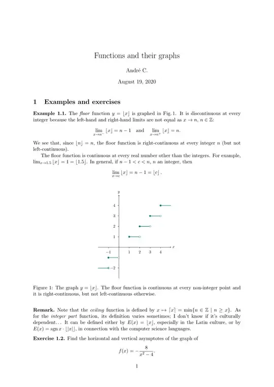
I'm doing graduation in math, and I've always been a keen observer of math writing (its punctuation, style). I've started learning LaTeX a couple of months ago, and here I'm presenting my document before experts to check it and provide me with their valuable suggestions and advice.

\documentclass[12pt, a4paper]{article}
\usepackage[margin=1in]{geometry}
\usepackage{amssymb}
\usepackage{amsmath}
\usepackage{amsthm}
\usepackage{tikz}
\usepackage{amssymb}
\renewcommand{\qed}{\tag*{$\blacksquare$}}
\newcommand{\QEDA}{\null\nobreak\hfill\ensuremath{\blacksquare}}
\newcommand{\QEDB}{\null\nobreak\hfill\ensuremath{\square}}
\pagestyle{empty}
\usepackage{enumitem}
\begin{document}
\noindent \textbf{Example 1}\hspace{24pt}The function $y=\lfloor x\rfloor$ is graphed in Figure 0.1. It is discontinuous at every integer because the left-hand and right-hand limits are not equal as $x\to\infty$:
[ \lim_{x\to n^-}\lfloor x\rfloor=n-1 \mbox{\hspace{12pt} and \hspace{12pt}} \lim_{x\to n^+}\lfloor x\rfloor=n. ]
\vspace{12pt}
\begin{center}
\begin{tikzpicture}[domain=-2:5, smooth]
\draw[->] (-2,0)--(5,0) node[right]{$x$};
\draw[->] (0,-3)--(0,5) node[above]{$y$};
\foreach \x in {-1, 1, 2, 3, 4} \draw (\x,0)--(\x,2pt) node[below=3pt]{$\x$};
\foreach \y in {-2,1,2,3,4} \draw (0,\y)--(2pt,\y) node[left=3pt]{$\y$};
\draw[color=blue!50!green, thick] (-2,-2)--(-1,-2);
\draw[color=blue!50!green,fill=white, thick] (-1,-2) circle (2pt);
\filldraw[color=blue!50!green,thick] (-1,-1) circle (2pt);
\draw[color=blue!50!green,thick] (-1,-1)--(0,-1);
\draw[color=blue!50!green,fill=white, thick] (0,-1) circle (2pt);
\filldraw[color=blue!50!green,thick] (0,0) circle (2pt);
\draw[color=blue!50!green,thick] (0,0)--(1,0);
\draw[color=blue!50!green,fill=white, thick] (1,0) circle (2pt);
\filldraw[color=blue!50!green,thick] (1,1) circle (2pt);
\draw[color=blue!50!green,thick] (1,1)--(2,1);
\draw[color=blue!50!green,fill=white, thick] (2,1) circle (2pt);
\filldraw[color=blue!50!green,thick] (2,2) circle (2pt);
\draw[color=blue!50!green,thick] (2,2)--(3,2);
\draw[color=blue!50!green,fill=white, thick] (3,2) circle (2pt);
\filldraw[color=blue!50!green,thick] (3,3) circle (2pt);
\draw[color=blue!50!green,thick] (3,3)--(4,3);
\draw[color=blue!50!green,fill=white, thick] (4,3) circle (2pt);
\filldraw[color=blue!50!green,thick] (4,4) circle (2pt);
\draw[color=blue!50!green,thick] (4,4)--(5,4);
\draw (2.5,2.5) node[left]{$y=\lfloor x\rfloor$};
\end{tikzpicture}
\end{center}
\begin{quote}
\small{\textsc{Figure 0.1}\hspace{18pt}The greatest integer function is continuous at every noninteger point. It is right-continuous, but not left-continuous, at every integer point.}
\end{quote}
\vspace{12pt}
Since $\lfloor n\rfloor=n$, the greatest integer function is right-continuous at every integer $n$ (but not left-continuous).
The greatest integer function is continuous at every real number other than the integers. For example,
[ \lim_{x\to1.5}\lfloor x\rfloor=1=\lfloor 1.5\rfloor. ]
In general, if $n-1<c<n$, $n$ an integer, then
[ \lim_{x\to c}\lfloor x\rfloor=n-1=\lfloor c\rfloor. \qed ]
\vspace{12pt}
\noindent\textbf{Example 2}\hspace{24pt}Find the horizontal and vertical asymptotes of the graph of
[ f(x)=-\frac{8}{x^2-4}. ]
\noindent\textbf{Solution}\hspace{24pt}We are interested in the behavior as $x\to\pm\infty$ and as $x\to\pm2$, where the denominator is zero. Notice that $f$ is an even functionof $x$, so its graph is symmetric with respect to the $y$-axis.
\begin{enumerate}[wide, labelwidth=!, labelindent=0pt]
\item[\textbf{(a)}]
\emph{The behavior as $x\to\pm\infty$}. Since $\lim_{x\to\infty}f(x)=0$, the line $y=0$ is a horizontal asymptote of the graph to the right. By symmetry it is an asymptote to the left as well (Figure 0.2). Notice that the curve approaches the $x$-axis from only the negative side (or from below). Also, $f(0)=2$.\
\item[\textbf{(b)}]
\emph{The behavior as $x\to\pm2$}. Since
[ \lim_{x\to2^+}f(x)=-\infty \hspace{24pt}\mbox{ and }\hspace{24pt} \lim_{x\to2^-}f(x)=\infty, ]
the line $x=2$ is a vertical asymptote bith from the right and from the left. By symmetry, the line $x=-2$ is also a vertical asymptote.
\end{enumerate}
There are no other asymptotes because $f$ has a finite limit at every other point.\QEDA
\vspace{12pt}
\begin{center}
\begin{tikzpicture}[domain=-5:5, smooth]
\draw[->] (-7,0)--(7,0) node[right]{$x$};
\draw[->] (0,-4.5)--(0,9) node[above]{$y$};
\drawcolor=red, thick--(2,-4.3);
\drawcolor=red, thick--(-2,-4.3);
\drawcolor=red, thick--(5.5,0);
\foreach \x in {-4,-3,-2,-1, 0, 1, 2, 3, 4} \draw (\x,0)--(\x,2pt) node[below=3pt, fill=white]{$\x$};
\foreach \y in {1,2,3,4,5,6,7,8} \draw (0,\y)--(2pt,\y) node[left=3pt]{$\y$};
\foreach \y in {-4,-3,-2,-1} \draw (0,\y)--(2pt,\y);
\draw[color=blue!50!green, thick] (-1.9,8) .. controls (-1.88,6) and (-1.7,2.1) .. (0,2);
\draw[color=blue!50!green, thick] (1.9,8) .. controls (1.88,6) and (1.7,2.1) .. (0,2);
\draw[color=blue!50!green, thick] (5.5, -0.2) .. controls (3, -0.3) and (2.3, -1) .. (2.2, -4.3);
\draw[color=blue!50!green, thick] (-5.5, -0.2) .. controls (-3, -0.3) and (-2.3, -1) .. (-2.2, -4.3);
\draw (2,7) node[right=12pt, fill=white]{$ \displaystyle y=-\frac{8}{x^2-4} $};
\draw (2,4) node[right]{Vertical asymptote, $x=2$};
\draw (-2,4) node[left]{Vertical asymptote, $x=-2$};
\draw[thin] (2.5,0)--(3, 0.8) node[above right]{Horizontal asymptote, $y=0$};
\end{tikzpicture}
\end{center}
\begin{quote}
\small{\textsc{Figure 0.2}\hspace{18pt}Graph of the function in Example 2.
 Notice that the curve approaches the $x$-axis from only one side.
Asymptotes do not have to be two sided.}
\end{quote}
\vspace{12pt}
\noindent \textbf{Example 3}\hspace{24pt}Find the area of the region bounded by the curve $y=xe^{-x}$ and the $x$-axis from $x=0$ to $x=4$.
\vspace{12pt}
\noindent\textbf{Solution}\hspace{24pt}The region is shaded in Figure 0.3. Its area is
[ \int_{0}^{4}xe^{-x},dx. ]
\vspace{12pt}
\begin{center}
\begin{tikzpicture}[domain=-1:4.2, smooth, scale=2]
\draw[->] (-1.3, 0)--(4.5,0) node[right]{$x$};
\draw[->] (0, -1.3)--(0, 1.3) node[above]{$y$};
\draw (0,0) node[below left=2pt]{$0$};
\foreach \x in {-1, 1, 2, 3, 4} \draw (\x, 0)--(\x,2pt) node[below=6pt, fill=white]{$\x$};
\foreach \y in {-1, -0.5, 0.5, 1} \draw(0, \y)--(2pt, \y) node[left=5pt]{$\y$};
\clip (-0.8, -1.2) rectangle (4.5, 1);
\draw[color=purple, thick] plot(\x, {(\x)(e^(-\x))});
\clip(0,0) rectangle (4,1);
\fill[color=purple, opacity=0.3] plot(\x, {(\x)(e^(-\x))});
\draw (2,0) node[above=18pt]{$y=xe^{-x}$};
\end{tikzpicture}
\end{center}
\begin{center}
\small{\textsc{Figure 0.3}\hspace{18pt}The region in Example 3.}
\end{center}
\vspace{12pt}
Let $u=x$, $dv=e^{-x}$, $v=-e^{-x}$, and $du=dx$. Then,
\begin{align}
\int_{0}^{4}xe^{-x},dx&=\left.-xe^{-x}\right]{0}^{4}-\int{0}^{4}\left(-e^{-x}\right),dx\
&=\left[-4e^{-4}-(0)\right]+\int_{0}^{4}e^{-x},dx\
&=\left.-4e^{-4}-e^{-x}\right]_{0}^{4}\
&=-4e^{-4}-e^{-4}-(-e^0)=1-5e^{-4}\approx0.91.
\qed
\end{align}
\end{document}

Answer 1

In the file below I tried to exemplify @leandriis and David Carlisle's suggestions and remarks. I kept only the first two examples from your original file. I also made some other modifications (simplifying some code and trying to introduce LaTeX objects that may be needed when editing a math assignment or whatever).

It would be helpful to look at What are the most common mistakes that beginners of (La)TeX and Friends make? and at https://thinkscience.co.jp/en/articles/LaTeX-habits-to-avoid.

I'm not considering myself an expert, but I'll give two personal opinions (not so original I guess):

1. (LaTeX) Try to separate the style (mainly in the preamble) from the content, and let LaTeX do the formatting job. It is the main typographer after all.
2. (Math) Using the small square at the end of an example or exercise (why ending the list here) is a question of taste and yields long discussions. The original sense of the symbol is to indicate that a proof just ended. Maybe it should stay like this. (LaTeX automatically inserts a vertical space at the end of an example environment indicating its end. Two signals for this event are too many; like using more than one exclamation mark at the end of a phrase.)

\documentclass[12pt, a4paper]{article}
\usepackage[margin=1in]{geometry}
\usepackage{amssymb}
\usepackage{amsmath}
\usepackage{amsthm}
\usepackage{tikz}
\usepackage{enumitem}
\newtheorem{thm}{Theorem}[section]
\theoremstyle{definition}
\newtheorem{exa}[thm]{Example}
\newtheorem{exe}[thm]{Exercise}
\newtheorem{rem}[thm]{Remark}
\newtheorem{rem}{Remark}
\newcommand{\textq}[1]{\text{\quad#1\quad}}
\newcommand{\floor}[1]{\left\lfloor#1\right\rfloor}
\newcommand{\ceil}[1]{\left\lceil#1\right\rceil}
\newcommand{\sgn}{\operatorname{sgn}}
% \renewcommand{\qed}{\tag{$\blacksquare$}}
% \newcommand{\QEDA}{\null\nobreak\hfill\ensuremath{\blacksquare}}
% \newcommand*{\QEDB}{\null\nobreak\hfill\ensuremath{\square}}
% \pagestyle{empty}
\title{Functions and their graphes}
\author{Andr'e C.}
\begin{document}
\maketitle
\section{Examples and exercises}
\begin{exa}
The \emph{floor} function $y=\floor{x}$ is graphed in
Fig.,\ref{fig:intPart}.  It is discontinuous at every integer because
the left-hand and right-hand limits are not equal as $x\to n$,
$n\in\mathbb{Z}$:
[
  \lim_{x\to n^-}\floor{x}=n-1
  \textq{and}
  \lim_{x\to n^+}\floor{x}=n.
]
We see that, since $\lfloor n\rfloor=n$, the floor function is
right-continuous at every integer $n$ (but not left-continuous).
The floor function is continuous at every real number other
than the integers.  For example,
$\lim_{x\to1.5}\floor{x}=1=\floor{1.5}$.
In general, if $n-1<c<n$, $n$ an integer, then
[
  \lim_{x\to c}\floor{x}=n-1=\floor{c}.
]
\begin{figure}[ht!]
  \centering
  \begin{tikzpicture}[scale=.8, every node/.style={scale=.8}]
    \draw[->] (-2,0)--(5,0) node[right]{$x$};
    \draw[->] (0,-3)--(0,5) node[above]{$y$};
\foreach \x in {-1, 1, 2, 3, 4} \draw (\x,0) -- +(0,-3pt)
node[below=3pt]{$\x$};
\foreach \y in {-2,1,2,3,4} \draw (0,\y) -- +(-3pt,0)
node[left=3pt]{$\y$};

\begin{scope}[blue!50!green, thick]
  \draw (-2,-2) -- (-1,-2);
  \draw[fill=white] (-1,-2) circle (2pt);

  \foreach \x in {-1, 1, 2, 3}{%
    \filldraw (\x, \x) circle (2pt)
    -- +(1, 0) circle (2pt) node[circle, fill=white, inner sep=1.4pt] {};
  }

  \filldraw (4,4) circle (2pt) -- (5,4);
\end{scope}


\end{tikzpicture}
  \caption{The graph $y=\floor{x}$.  The floor function is continuous
    at every non-integer point and it is right-continuous, but not
    left-continuous otherwise.}
  \label{fig:intPart}
\end{figure}
\end{exa}
\begin{rem}
Note that the \emph{ceiling} function is defined by
$x\mapsto\ceil{x}=\min{n\in\mathbb{Z} \mid n\geq x}$.  As for the
\emph{integer part} function, its definition varies sometimes; I don't
know if it's culturally dependent\ldots\ It can be defined either by
$E(x)=\floor{x}$, especially in the Latin culture, or by
$E(x)=\sgn{x}\cdot\floor{|x|}$, in connection with the computer science
languages.
\end{rem}
\begin{exe}
  \label{e:graph}
Find the horizontal and vertical asymptotes of the graph of
[
  f(x)=-\frac{8}{x^2-4}.
]
\noindent
\emph{Solution}.
We are interested in the behavior of the graph as $x\to\pm\infty$ and
as $x\to\pm2$---where the denominator is zero.  Notice that $f$ is an
even function of $x$, so its graph is symmetric with respect to the
$y$-axis.
\begin{enumerate}[wide, labelindent=0pt, label={\textbf{(\alph*)}}]
\item
\emph{The behavior as $x\to\pm\infty$}. Since
$\lim_{x\to\infty}f(x)=0$, the line $y=0$ is a horizontal asymptote of
the graph to the right. By symmetry it is an asymptote to the left as
well (Figure 0.2). Notice that the curve approaches the $x$-axis from
only the negative side (or from below). Also, $f(0)=2$.
\item
\emph{The behavior as $x\to\pm2$}. Since
[
  \lim_{x\to2^+}f(x)=-\infty
  \textq{and}
  \lim_{x\to2^-}f(x)=\infty,
]
the line $x=2$ is a vertical asymptote bith from the right and from
the left. By symmetry, the line $x=-2$ is also a vertical asymptote.
\end{enumerate}
There are no other asymptotes because $f$ has a finite limit at every
other point.  The graph is shown in Fig.,\ref{fig:graph}.
\qed
\end{exe}
\begin{figure}[ht!]
  \centering
  \begin{tikzpicture}[every node/.style={scale=.8}]
    \draw[->, thin] (-7,0)--(7,0) node[right]{$x$};
    \draw[->, thin] (0,-4.5)--(0,9) node[above]{$y$};
\draw[color=red](2,8)--(2,-4.3);
\draw[color=red](-2,8)--(-2,-4.3);
\draw[color=red](-5.5,0)--(5.5,0);

\foreach \x in {-4,-3,-2,-1, 0, 1, 2, 3, 4}
\draw (\x,0)--(\x,2pt) node[below=3pt, fill=white]{$\x$};
\foreach \y in {1,2,3,4,5,6,7,8}
\draw (0,\y)--(2pt,\y) node[left=3pt]{$\y$};
\foreach \y in {-4,-3,-2,-1} \draw (0,\y)--(2pt,\y);

\draw[color=blue!50!green, thick]
(-1.9,8) .. controls (-1.88,6) and (-1.7,2.1) .. (0,2);
\draw[color=blue!50!green, thick]
(1.9,8) .. controls (1.88,6) and (1.7,2.1) .. (0,2);

\draw[color=blue!50!green, thick]
(5.5, -0.2) .. controls (3, -0.3) and (2.3, -1) .. (2.2, -4.3);
\draw[color=blue!50!green, thick]
(-5.5, -0.2) .. controls (-3, -0.3) and (-2.3, -1) .. (-2.2, -4.3);

\draw (2,4) node[right]{vertical asymptote, $x=2$};
\draw (-2,4) node[left]{vertical asymptote, $x=-2$};
\draw[gray, thin] (2.5, 2pt) to[out=80, in=180] (3, 0.8)
node[text=black, right] {horizontal asymptote, $y=0$};

\end{tikzpicture}
  \caption{Graph of the function $y=-\dfrac{8}{x^2-4}$.  Notice
    that the curve approaches the $x$-axis from only one side.
    Asymptotes do not have to be two sided.}
  \label{fig:graph}
\end{figure}
\end{document}