10

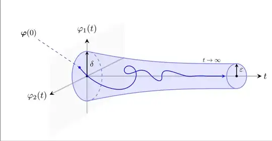
I am trying to recreate a trajectory plot to demonstrate stability. The image I have in mind is something similar to this following figure:

Asymptotic stability

The problem is, I do not really known how to generate the line trajectory, as I do not have any numerical data to rely on. The form of the trajectory is irrelevant as long as it shows asymptotic behavior. Preferably it should look like the one in the figure. I will attatch my current progress in the following code:

\documentclass[tikz]{standalone}
\usepackage{geometry}
\usepackage{pgfplots}
\usepackage{bm}
\usetikzlibrary{3d,calc}
\usepgfplotslibrary{fillbetween}

\begin{document} \begin{tikzpicture}%[show grid=all] % background \path[name path=C] (-1.5,1.75) -- (1.5,3.25); \path[name path=D] (-1.5,-1.5) -- (1.5,0.5); \tikzfillbetween[of=C and D]{top color=gray!10!white, bottom color=white, opacity=0.02}; % axis \draw[gray!50!white,->,very thick,>=latex] (0,-0.5) -- (0,2.5); \draw[gray!50!white,->,very thick,>=latex] (1.5,1.75) -- (-1.5,0.25); \draw[gray!50!white,->,very thick,>=latex] (0,1) -- (7,1); \filldraw[black] (0,1) circle (1.2pt); \filldraw[black] (6,1) circle (1.2pt); \draw[blue!50!white,dashed,very thick] (0,0) arc (-90:90:0.6cm and 1cm); \draw[blue!50!white,thick] (0,0) arc (-90:90:-0.6cm and 1cm); \draw[blue!50!white,thick] (6,0.5) arc (-90:90:-0.4cm and 0.5cm); \draw[blue!50!white,thick] (6,0.5) arc (-90:90:0.4cm and 0.5cm); \draw[blue!50!white,thick,name path = A] (0,2) to[in=180,out=-12] (6,1.5); \draw[blue!50!white,thick,name path = B] (0,0) to[in=180,out=12] (6,0.5); \tikzfillbetween[of=A and B]{blue!50!white, opacity=0.2}; \shade[left color=blue!50!white,right color=blue!50!white,opacity=0.2] (0,0) arc (-90:90:-0.6cm and 1cm); \shade[left color=blue!50!white,right color=blue!50!white,opacity=0.2] (6,0.5) arc (-90:90:0.4cm and 0.5cm); % axis labels \node at (0,2.9) {$\varphi_{1}(t)$}; \node at (-2,0.21) {$\varphi_{2}(t)$}; \node at (7.15,1) {$t$}; \draw[thick,->,>=latex] (0,1) -- (0,2) node [midway,scale=0.9,right]{$\delta$}; \draw[thick,->,>=latex] (6,1) -- (6,1.5) node [midway,scale=0.9,right]{$\varepsilon$}; \draw[dashed,blue] (-0.3,1.35) -- (-2,2.5) node [pos=1.2,text=black,scale=0.9]{$\bm{\varphi}(0)$}; % trajectory \filldraw[blue!90!white] (-0.3,1.35) circle (1.2pt); % border adjustment (standalone crop problems) \node at (0,-2.3) {$$}; \node at (8,0) {$$}; \end{tikzpicture} \end{document}

Current progress

Bakr
  • 499

1 Answers1

7

I was able to use the answer from Plotting loops: trajectories and directions to plot the following trajectory: enter image description here

Here is the code:

\documentclass[tikz]{standalone}
\usepackage{geometry}
\usepackage{pgfplots}
\usepackage{bm}
\usetikzlibrary{3d,calc}
\usepgfplotslibrary{fillbetween}
\usetikzlibrary{arrows.meta,hobby}

\begin{document} \begin{tikzpicture}[use Hobby shortcut]%[show grid=all] \tikzset{axisArrow/.style={gray!50!white,very thick,>=stealth,arrows={->[fill=black]}}} % background \path[name path=C] (-1.5,1.75) -- (1.5,3.25); \path[name path=D] (-1.5,-1.5) -- (1.5,0.5); \tikzfillbetween[of=C and D]{top color=gray!10!white, bottom color=white, opacity=0.02}; % axis \draw[axisArrow] (0,-0.5) -- (0,2.5); \draw[axisArrow] (1.5,1.75) -- (-1.5,0.25); \draw[axisArrow] (0,1) -- (7,1); \filldraw[black] (0,1) circle (1.2pt); \filldraw[black] (6,1) circle (1.2pt); \draw[blue!50!white,dashed, thick] (0,0) arc (-90:90:0.6cm and 1cm); \draw[blue!50!white,thick] (0,0) arc (-90:90:-0.6cm and 1cm); \draw[blue!50!white,thick] (6,0.5) arc (-90:90:-0.4cm and 0.5cm); \draw[blue!50!white,thick] (6,0.5) arc (-90:90:0.4cm and 0.5cm); \draw[blue!50!white,thick,name path = A] (0,2) to[in=180,out=-12] (6,1.5); \draw[blue!50!white,thick,name path = B] (0,0) to[in=180,out=12] (6,0.5); \tikzfillbetween[of=A and B]{blue!50!white, opacity=0.2}; \shade[left color=blue!50!white,right color=blue!50!white,opacity=0.2] (0,0) arc (-90:90:-0.6cm and 1cm); \shade[left color=blue!50!white,right color=blue!50!white,opacity=0.2] (6,0.5) arc (-90:90:0.4cm and 0.5cm); % axis labels \node at (0,2.9) {$\varphi_{1}(t)$}; \node at (-2,0.21) {$\varphi_{2}(t)$}; \node at (7.15,1) {$t$}; \node[scale=0.7] at (5,1.65) {$t\rightarrow \infty$}; \draw[thick,->,>=stealth] (0,1) -- (0,2) node [midway,scale=0.9,right]{$\delta$}; \draw[thick,->,>=stealth] (6,1) -- (6,1.5) node [midway,scale=0.9,right]{$\varepsilon$}; \draw[dashed,blue] (-0.3,1.35) -- (-2,2.5) node [pos=1.2,text=black,scale=0.9]{$\bm{\varphi}(0)$}; % trajectory \filldraw[blue!90!white] (-0.3,1.35) circle (1.2pt); \draw[-stealth,blue!90!white,thick] (-0.3,1.35) .. (1,0.5) .. (1.75,1.4) .. (1.5,1.2) .. (2,1.2) .. (2.5,1.1) .. (3,0.9) .. (3,1) .. (4,1) .. (4.3,1) .. (4.8,1) -- (5.55,1); % border adjustment (standalone crop problems) \node at (0,-2.3) {$$}; \node at (8,0) {$$}; \end{tikzpicture} \end{document}

Bakr
  • 499