Tangent vector to curve

Question

Code:

\documentclass[12pt]{article}
\usepackage{pgfplots}
\usepackage{tikz}
\usetikzlibrary{shapes,arrows}
\usetikzlibrary{decorations.markings}
\usepackage[margin=1in]{geometry}
\begin{document}
    \begin{figure}[h!]
        \centering
        \begin{tikzpicture}
            \begin{axis}[view={120}{20},
                height = 4in,width=4in,
                axis lines=center,axis on top,
              no marks,axis equal,
                xmin=-1.5,xmax=1.5,ymin=-1.5,ymax=1.5,zmin=-1.5,zmax=1.5,
             enlargelimits={upper=0.1}]
                    \addplot3+[color = blue, thick, no markers,samples=250, samples y=0,domain=0:2pi,variable=\t, decoration={
    markings,
    mark=between positions 0.01 and .999 step 2em with {\arrow [scale=1]{stealth}}
    }, postaction=decorate]({sin(\t r)},{sin(2\t r)},{sin(3\t r)});
                    \draw[color = red, very thick,-latex] ({sin(3 r)}, {sin(6 r)}, {sin(9 r)}) -- ++({cos(3 r)}, {2cos(6 r)}, {3*cos(9 r)});
            \end{axis}
        \end{tikzpicture}

    \end{figure}
\end{document}

Plot:

How to properly draw a line tangent to the curve at t = 2?

Answer 1

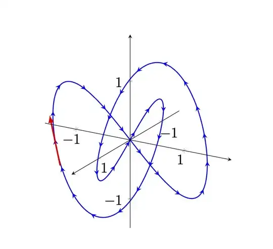
You are already placing tons of tangent arrow heads, so you can use the same strategy to place a complete arrow in a second postaction. Since t runs from 0 to 2pi and you want to place the arrow at t=2, the position is 1/pi. Please note that it is important to use coordinates with units, i.e.

\draw[color = red, very thick,-latex]  (-0.5cm,0cm) -- (0.5cm,0cm);

to have the arrow parallel since otherwise you will be using a coordinate system installed by pgfplots.

\documentclass[12pt]{article}
\usepackage{pgfplots}
\pgfplotsset{compat=1.17}
\usetikzlibrary{decorations.markings}
\usepackage[margin=1in]{geometry}
\begin{document}
    \begin{figure}[h!]
        \centering
        \begin{tikzpicture}
            \begin{axis}[view={120}{20},
                height = 4in,width=4in,
                axis lines=center,axis on top,
              no marks,axis equal,
                xmin=-1.5,xmax=1.5,ymin=-1.5,ymax=1.5,zmin=-1.5,zmax=1.5,
             enlargelimits={upper=0.1}]
    \addplot3+[color = blue, thick, no markers,samples=250, samples y=0,domain=0:2pi,variable=\t, 
    postaction={decorate,decoration={
    markings,
    mark=between positions 0.01 and .999 step 2em with {\arrow [scale=1]{stealth}},
    }},
    postaction={decorate,decoration={
    markings,
    mark=at position 1/pi with {
        \draw[color = red, very thick,-latex] 
    (-0.5cm,0cm) -- (0.5cm,0cm);
    }
    }}
    ]({sin(deg(\t))},{sin(deg(2\t))},{sin(deg(3*\t))});
        \end{axis}
    \end{tikzpicture}   
\end{figure}

\end{document}

You can compute the velocity at a given t. (In principle you can compute the tangent analytically, too, so this hybrid answer is a bit senseless but this is a LaTeX answer so we let LaTeX find out the slope. We could also let it find out the velocity numerically, perhaps on another day. And of course the position is just an approximation, too.)

\documentclass[tikz,border=3mm]{standalone}
\usepackage{pgfplots}
\pgfplotsset{compat=1.17}
\usetikzlibrary{decorations.markings}
\begin{document}
\foreach \myt in {0.2,0.4,...,6.2}        
{\begin{tikzpicture}        
  \begin{axis}[view={120}{20},
                height = 4in,width=4in,
                axis lines=center,axis on top,
              no marks,axis equal,
                xmin=-1.5,xmax=1.5,ymin=-1.5,ymax=1.5,zmin=-1.5,zmax=1.5,
             enlargelimits={upper=0.1}]
    \addplot3+[color = blue, thick, no markers,samples=250, samples y=0,domain=0:2*pi,variable=\t, 
    postaction={decorate,decoration={
    markings,
    mark=between positions 0.01 and .999 step 2em with {\arrow [scale=1]{stealth}},
    }},
    postaction={decorate,decoration={
    markings,
    mark=at position {\myt/2/pi} with {
        \pgfmathsetmacro{\mylen}{sqrt(pow(cos(deg(\myt)),2)+pow(2*cos(deg(2*\myt)),2)+pow(3*cos(3*deg(\myt)),2))}
        \draw[color = red, very thick,-latex,overlay] 
    (0cm,0cm) -- (0.5*\mylen*1cm,0cm);
    }
    }}
    ]({sin(deg(\t))},{sin(deg(2*\t))},{sin(deg(3*\t))});
\end{axis}
\end{tikzpicture}}
\end{document}