pgf: "Dimension too large" in a function which fits into a graph, /pgf/fpu=true does not help

Question

I want to plot a lognormal function:

\documentclass{article}
\usepackage{pgfplots}
\begin{document}

\pgfmathdeclarefunction{lognormal}{2}{%
%  \pgfkeys{/pgf/fpu=true}
  \pgfmathparse{1/(x#2sqrt(2pi))exp(-((ln(x)-#1)^2)/(2*#2^2))}%
%  \pgfmathresult
%  \pgfkeys{/pgf/fpu=false}
}
\begin{tikzpicture}
\begin{axis}[ domain=0.01:10 ]
  \addplot {lognormal(ln(5),0.02)};
\end{axis}
\end{tikzpicture}
\end{document}

It produces "Dimension too large" even that the function has moderate values. I guess that the problem lies in intermediate values within exp(). I tried /pgf/fpu=true (commented out in the source) as suggested in this answer but it did not help and even additionally confused PGF. The latter can be verified by replacing lognormal(ln(5),0.02) with lognormal(ln(5),1).

How to draw the lognormal function in pgf? I tried to replace the problematic parts of the domain with y ~ 0:

\pgfmathparse{1/(x*#2*sqrt(2*pi))*exp(ifthenelse((ln(x)-#1)/sqrt(#2) < -10, -100, -((ln(x)-#1)^2)/(2*#2^2)))}

As seen, I do not use a square in the condition in order to avoid an overflow. However, for certain parameters, processing a single chart with that equation takes several seconds, and of the whole Tex document, with many charts, more than a minute. Is there a faster, more precise and more elegant solution?

Answer 1

Edit2:

The small wrapper made its way to CTAN. So the below code with an up to date LaTeX distribution is now just:

\documentclass{article}
\usepackage{pgfplots}
\usepackage{pgfmath-xfp}
\pgfmxfpdeclarefunction{lognormal}{3}
  {exp(-((ln(#1) - #2)^2) / (2 * (#3)^2)) / (#1 * #3 * sqrt(2 * pi))}
\begin{document}

\begin{tikzpicture}
\begin{axis}[ domain=0.01:10, samples=100 ]
  \addplot {lognormal(x,ln(5),0.02)};
\end{axis}
\end{tikzpicture}
\end{document}

Edit:

I've created a small wrapper to define pgfmath-functions using l3fp first posted here. With it the MWE here boils down to the following (the things between \ExplSyntaxOn and \ExplSyntaxOff is the wrapper):

\documentclass{article}
\usepackage{pgfplots}
\ExplSyntaxOn
\tl_new:N \l_pgffpeval_function_body_tl
\tl_new:N \l_pgffpeval_function_definition_tl
\int_new:N \l_pgffpeval_tmp_int
\cs_new_protected:Npn \pgffpeval_declare_function:nnn #1#2#3
  {
    __pgffpeval_initialize_body:
    \int_step_inline:nn {#2}
      {
        \tl_put_right:Nx \l_pgffpeval_function_body_tl
          {
            \exp_not:n { \pgfmathsetmacro } \exp_not:c { __pgffpeval_arg##1 }
              { \exp_not:n {####} ##1 }
          }
      }
    __pgffpeval_define_function:nnnn {#2} {#1} {#2} {#3}
  }
\cs_new_protected:Npn \pgffpeval_declare_function_processed_args:nnnn #1#2#3#4
  {
    __pgffpeval_initialize_body:
    \int_zero:N \l_pgffpeval_tmp_int
    \clist_map_inline:nn {#3}
      {
        \int_incr:N \l_pgffpeval_tmp_int
        \tl_put_right:Nx \l_pgffpeval_function_body_tl
          {
            \exp_not:n { \pgfmathsetmacro }
              \exp_not:c { __pgffpeval_arg \int_use:N \l_pgffpeval_tmp_int }
              { \exp_not:n {##1} }
          }
      }
    \exp_args:NV
    __pgffpeval_define_function:nnnn \l_pgffpeval_tmp_int {#1} {#2} {#4}
  }
\cs_new_protected:Npn __pgffpeval_initialize_body:
  {
    \tl_set:Nn \l_pgffpeval_function_body_tl
      {
        \group_begin:
        \pgfkeys{/pgf/fpu=true, /pgf/fpu/output~format=sci}%
      }
  }
\cs_new:Npn __pgffpeval_process_function_aux:n #1 { \exp_not:n {## #1} }
\cs_new_protected:Npn __pgffpeval_process_function:nnn #1#2#3
  {
    \exp_last_unbraced:Nx
    \cs_set_protected:cpn
      {
        { __pgffpeval_function_ #2 cmd }
        \int_step_function:nN {#1} __pgffpeval_process_function_aux:n
      }
      { \group_end: \exp_args:Nf \pgfmathparse { \fp_eval:n {#3} } }
  }
\cs_new_protected:Npn __pgffpeval_define_function:nnnn #1#2#3#4
  {
    __pgffpeval_process_function:nnn {#1} {#2} {#4}
    \tl_put_right:Nx \l_pgffpeval_function_body_tl
      {
        \use:x
          { 
            \exp_not:c { __pgffpeval_function #2 _cmd }
            \int_step_function:nN {#1} __pgffpeval_define_function_aux:n
          }
      }
    \exp_args:Nnno
    \pgfmathdeclarefunction {#2} {#3} \l_pgffpeval_function_body_tl
  }
\cs_new:Npn __pgffpeval_define_function_aux:n #1
  { { \exp_not:c { __pgffpeval_arg#1 } } }
\NewDocumentCommand \pgfmathdeclarefpevalfunction { m m o m }
  {
    \IfValueTF {#3}
      { \pgffpeval_declare_function_processed_args:nnnn {#1} {#2} {#3} }
      { \pgffpeval_declare_function:nnn {#1} {#2} }
      {#4}
  }
\ExplSyntaxOff
\pgfmathdeclarefpevalfunction{lognormal}{3}
  {exp(-((ln(#1) - #2)^2) / (2 * (#3)^2)) / (#1 * #3 * sqrt(2 * pi))}
\begin{document}

\begin{tikzpicture}
\begin{axis}[ domain=0.01:10, samples=100 ]
  \addplot {lognormal(x,ln(5),0.02)};
\end{axis}
\end{tikzpicture}
\end{document}

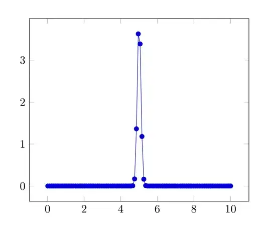
Output and explanation like below.

---

The following uses xfp for the actual calculation, and \pgfmathsetmacro with the options /pgf/fpu=true and /pgf/fpu/output format=sci applied locally to ensure the input number format is understandable for xfp (as pgfmath uses a custom internal number representation when the FPU is used, which isn't understood by xfp).

The \romannumeral is used to ensure that \fpeval is fully done when the group is closed and therefore \argA, \argB, and \argC don't have the correct meaning anymore. The result is then again parsed by \pgfmathparse to make sure that \pgfmathresult holds the correct format for pgf outside of the function.

\documentclass{article}
\usepackage{pgfplots}
\usepackage[]{xfp}
\begin{document}

\pgfmathdeclarefunction{lognormal}{3}{%
  \begingroup
    \pgfkeys{/pgf/fpu=true, /pgf/fpu/output format=sci}%
    \pgfmathsetmacro\argA{#1}%
    \pgfmathsetmacro\argB{#2}%
    \pgfmathsetmacro\argC{#3}%
    \expandafter
  \endgroup
  \expandafter\pgfmathparse\expandafter
    {%
      \romannumeral`^^@%
      \fpeval{exp(-((ln(\argA)-\argB)^2)/(2\argC^2))/(\argA\argCsqrt(2pi))}%
    }%
}
\begin{tikzpicture}
\begin{axis}[ domain=0.01:10, samples=100 ]
  \addplot {lognormal(x,ln(5),0.02)};
\end{axis}
\end{tikzpicture}
\end{document}

Is it fast? No. Does it work? Yes: