Plotting resistance and reactance curves on the Smith Chart

Question

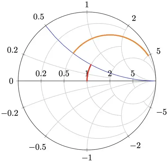
For my class, I have been trying to plot constant resistance and reactance curves on the Smith chart. While the latter appears to be straightforward, the only way I can think of for the former is plotting a group of closely spaced points, which becomes quite memory intensive. My questions are:

1. Is there any way efficient way to plot constant resistance curves (red and orange in this case), like the reactance curve (blue)?
2. Is there a way to shift the originating point of the blue (reactance) curve to a point say the one intersecting with the red one?

After following the answers from here and here, I have arrived at:

\documentclass[preview]{standalone}
\usepackage{tikz}
\usepackage{pgfplots}
\usepgfplotslibrary{smithchart}
\pgfplotsset{compat=1.11}
\begin{document}
    \begin{tikzpicture}
        \begin{smithchart}
    % Reactance plot
    \addplot[domain=0:90, samples=600, color=blue] {.5};

    % Resistance plot - orange 
    \foreach \x in {.5, .51,...,5}
    {\edef\temp{\noexpand\addplot+[mark=*,
    mark options={solid},color={orange},mark size=.2,line width=1] coordinates { (.5,\x) };}\temp}

    % Resistance plot - red 
    \foreach \x in {0, .01,...,.5}
    {\edef\temp{\noexpand\addplot+[mark=*,
    mark options={solid},color={red},mark size=.2,line width=1] coordinates { (1,\x) };}\temp}

    \end{smithchart}
\end{tikzpicture}

\end{document}

which generates the output below:

Thanks!

Answer 1

I do not really understand the question. However, one of your concerns seems to be compilation time. This code reproduces your output in a fraction of time. (Using \pgfplotsinvokeforeach without the \edef stuff already speeds it up quite a bit, but the following is even faster.)

\documentclass[preview]{standalone}
\usepackage{pgfplots}
\usepgfplotslibrary{smithchart}
\pgfplotsset{compat=1.17}
\begin{document}
    \begin{tikzpicture}
        \begin{smithchart}
    % Reactance plot
    \addplot[domain=0:90, samples=600, color=blue] {.5};

    % Resistance plot - orange 
    \addplot+[mark=*,only marks,samples at={.5, .51,...,5},
    mark options={solid},color={orange},mark size=.2,line width=1](.5,x) ;

    % Resistance plot - red 
    \addplot+[mark=*,only marks,samples at={0, .01,...,.5},
    mark options={solid},color={red},mark size=.2,line width=1] (1,x) ;

    \end{smithchart}
\end{tikzpicture}

\end{document}

But I really do not understand why you do not do something like

\documentclass[preview]{standalone}
\usepackage{pgfplots}
\usepgfplotslibrary{smithchart}
\pgfplotsset{compat=1.17}
\begin{document}
    \begin{tikzpicture}
        \begin{smithchart}[samples=181,line cap=round,smooth]
    % Reactance plot
    \addplot[domain=0:20,  color=blue] (x,.5);

    % Resistance plot - orange 
    \addplot+[no marks,domain=.5:5,
    color={orange},line width=1](.5,x) ;

    % Resistance plot - red 
    \addplot+[no marks,domain=0:.5,
        color={red},line width=1] (1,x) ;

    \end{smithchart}
\end{tikzpicture}

\end{document}