14

I need to draw the border of a generic region in tikz. A code with this idea is presented below.

\documentclass{standalone}
\usepackage[utf8]{inputenc}
\usepackage{tikz}
\usepackage{color,xcolor}
\begin{document}
\begin{tikzpicture}
\draw[-latex] (-0.5,0) -- (6,0) node[right]{$x_1$};
\draw[-latex] (0,-0.5) -- (0,6) node[above]{$x_2$};
\draw [fill=cyan,opacity=0.5] plot [smooth cycle,tension=0.5] coordinates {(0.38,4.74) (0.78,3.54) (2.16,2.88) (2.88,1.54) (4.18,0.8) (5.38,0.82) (6.02,2.32) (6.02,3.66) (5.3,5.04) (3.68,5.44) (1.82,5.52)};
\draw[red,thick] plot [smooth,tension=0.5] coordinates {(0.38,4.74) (0.78,3.54) (2.16,2.88) (2.88,1.54) (4.18,0.8)};
\end{tikzpicture}
\end{document}

whose output is the following:

enter image description here

However, when I repeat the coordinates of the boundary, it seems that the red line does not fit the region, even when I change the tension parameter.

How can I solve this?

7 Answers7

12

You can draw it twice but with a clipping rectangle for the second.

\documentclass{standalone}
\usepackage[utf8]{inputenc}
\usepackage{tikz}
\usepackage{color,xcolor}
\begin{document}
\begin{tikzpicture}
\draw[-latex] (-0.5,0) -- (6,0) node[right]{$x_1$};
\draw[-latex] (0,-0.5) -- (0,6) node[above]{$x_2$};
\draw [fill=cyan,opacity=0.5] plot [smooth cycle,tension=0.5] coordinates {(0.38,4.74) (0.78,3.54) (2.16,2.88) (2.88,1.54) (4.18,0.8) (5.38,0.82) (6.02,2.32) (6.02,3.66) (5.3,5.04) (3.68,5.44) (1.82,5.52)};
\begin{scope}
\clip (0.3,4.8) rectangle (4.20,0.15);
\draw[red,thick] plot [smooth cycle,tension=0.5] coordinates {(0.38,4.74) (0.78,3.54) (2.16,2.88) (2.88,1.54) (4.18,0.8) (5.38,0.82) (6.02,2.32) (6.02,3.66) (5.3,5.04) (3.68,5.44) (1.82,5.52)};
\end{scope}
\end{tikzpicture}
\end{document}

enter image description here

Ignasi
  • 136,588
12

Here is an alternative with blank from the hobby package:

\documentclass[tikz, border=1cm]{standalone}
\usetikzlibrary{hobby}
\begin{document}
\begin{tikzpicture}[use Hobby shortcut]
\draw[fill=cyan, opacity=0.5, closed, tension=10]  (0.38,4.74)..(0.78,3.54)..(2.16,2.88)..(2.88,1.54)..(4.18,0.8)..(5.38,0.82)..(6.02,2.32)..(6.02,3.66)..(5.3,5.04)..(3.68,5.44)..(1.82,5.52);
\draw[red, thick, closed, tension=10]   (0.38,4.74)..(0.78,3.54)..(2.16,2.88)..(2.88,1.54)..(4.18,0.8)..([blank]5.38,0.82)..([blank]6.02,2.32)..([blank]6.02,3.66)..([blank]5.3,5.04)..([blank]3.68,5.44)..([blank]1.82,5.52);
\end{tikzpicture}
\end{document}

Cyan shape with partly red border

It is not the same shape as before though. Hobby produces a smoother curve than plot - by design of the package/algorithm.

Edit: I now see that it seems that I completely stole the idea from the comments by @Andrew Stacey. Andrew is indeed the author of the brilliant package/implementation of Hobby. He might have an even better way to do this. My idea/starting point came from an old answer by me: https://tex.stackexchange.com/a/646711/8650

Edit: Code with fewer points, and reuse of path, but no fill yet - need to figure it out. (OK - fill can not be done when reusing the path)

\documentclass[tikz, border=1cm]{standalone}
\usetikzlibrary {decorations.pathreplacing, arrows.meta}
\usetikzlibrary{hobby}
\begin{document}
\begin{tikzpicture}[use Hobby shortcut]
\draw[red, thick,closed]  (0.4,4.0)..(2.2,2.9)..(2.9,1.5)..(4.3,0.8)..([blank=soft]5.4,0.8)..([blank=soft]6.0,3)..([blank=soft]5.3,5.0)..([blank=soft]3.5,5.4)..([blank=soft]1.8,5.5);
\draw[cyan, use previous Hobby path={invert soft blanks, disjoint}] ;
\end{tikzpicture}
\end{document}

Unfilled shape part cyan and part red

  • 3
    +1. Even if my comment had actually had any detail and you'd seen it, I never consider fleshing out a comment to an answer to be stealing! It's being helpful. In addition, the nicest thing for me as a package author is to see others use my packages in answers. This is indeed the approach I was thinking about, I wondered if the OP would be happier with fewer defining points as the hobby package gives better shapes than the smooth style does. Also, it might be a good showcase for reusing a hobby path to avoid running the algorithm twice. – Andrew Stacey Sep 07 '22 at 23:42
  • @AndrewStacey: I have looked at the manual again, and I found that I am not really using the blank=soft function in the above code. I could just have used blank. I do not know how to reuse a path. I can save a path including blank=soft. The soft blanks can be inverted with invert soft blanks, but how do I ignore soft blanks? – hpekristiansen Sep 08 '22 at 00:35
  • 1
    You're absolutely right - it can't be done with the soft blank concept as is. Feels like a sensible thing to want to do so I'll have a think about how to extend the syntax to allow for this scenario. Your original method is therefore the best for the moment. (But I would be interested in seeing if one could get away with fewer points and still be close enough to the original curve - that's sort of the reason for hobby's algorithm) – Andrew Stacey Sep 08 '22 at 06:01
  • Maybe an ignore soft blanks option for future versions? I all ready added a version with fewer points, but it is hard to know if OP is happy with any Γ shape and if the red line is to end at specific points. – hpekristiansen Sep 08 '22 at 06:17
  • https://github.com/loopspace/hobby/issues/10 – Andrew Stacey Sep 08 '22 at 17:48
9

When PGF/TikZ plots a smooth curve through your coordinates it uses Bézier curves (as for all curves, including arcs, circles and ellipses). This curve needs two support points.

When you ask for a smooth or smooth cycled plot, these support points are calculated from the previous and the next points, the manual states:

In order to determine the control points of the curve at the point y, the handler computes the vector z − x and scales it by the tension factor (see below). Let us call the resulting vector s. Then y + s and y − s will be the control points around y.

For the smooth cycle plot the last coordinate will be the previous point for the first point and the first point will be the next point for the last point. However, for smooth the manual says:

The first control point at the beginning of the curve will be the beginning itself, once more; likewise the last control point is the end itself.

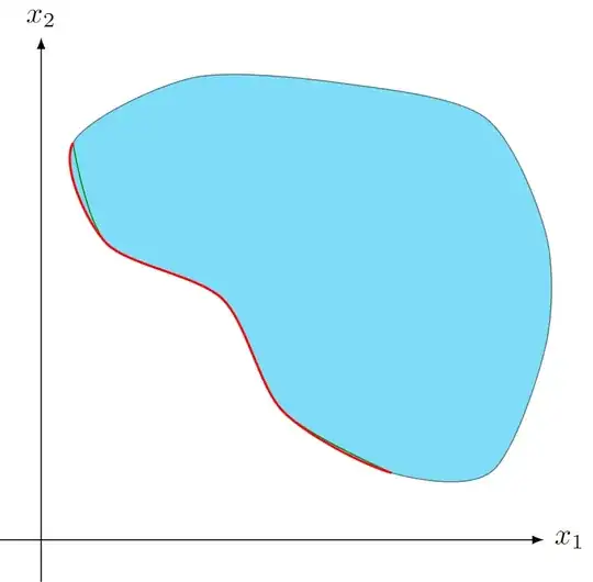
This is why your smooth plot is not equal to your closed plot on the first and last segment. It's missing the information about the very first previous and the very last next point.

With the decorations.pathreplacing library we can even inspect the the support points:

enter image description here

We need the red X that's on (0.38, 4.74) to be on the blue X left below of it to draw the same curve:

enter image description here


For this, I propose a slightly altered plothandler that uses the first and the last point to calculate the support points but does not draw any lines or curves to these points.

For this, I declare a plothandler \pgfplothandlercurvetostartend. In TikZ, this is mapped to the key smooth start and end.

You only need to supply the points to the plot yourself:

\draw[red,thick]
  plot [smooth start and end, tension=0.5]
    coordinates {
      (1.82,5.52) % coordinate before first
      (0.38,4.74) (0.78,3.54) (2.16,2.88) (2.88,1.54) (4.18,0.8)
      (5.38,0.82) % coordinate after last
    };

Code

\documentclass[tikz]{standalone}
\makeatletter
\tikzset{smooth start and end/.code={%
  \let\tikz@plot@handler=\pgfplothandlercurvetostartend}}
\pgfdeclareplothandler{\pgfplothandlercurvetostartend}{}{
  point macro=\pgf@plot@curvetostartend@handler@initial,
  jump macro=\pgf@plot@smoothstartend@next@moveto}
\def\pgf@plot@smoothstartend@next@moveto{%
  \global\pgf@plot@startedfalse
  \global\let\pgf@plotstreampoint\pgf@plot@curvetostartend@handler@initial}
\def\pgf@plot@curvetostartend@handler@initial#1{%
  \pgf@process{#1}%
  \xdef\pgf@plot@curveto@first{\noexpand\pgfqpoint{\the\pgf@x}{\the\pgf@y}}%
  \global\let\pgf@plot@curveto@first@support=\pgf@plot@curveto@first
  \global\let\pgf@plotstreampoint=\pgf@plot@curvetostartend@handler@second}
\def\pgf@plot@curvetostartend@handler@second#1{%
  \pgf@process{#1}%
  \xdef\pgf@plot@curveto@second{\noexpand\pgfqpoint{\the\pgf@x}{\the\pgf@y}}%
  \pgf@plot@first@action{\pgf@plot@curveto@second}%
  \global\let\pgf@plotstreampoint=\pgf@plot@curvetostartend@handler@third}
\def\pgf@plot@curvetostartend@handler@third#1{%
  \pgf@process{#1}%
  \xdef\pgf@plot@curveto@current{\noexpand\pgfqpoint{\the\pgf@x}{\the\pgf@y}}%
  % compute difference vector:
  \pgf@xa=\pgf@x
  \pgf@ya=\pgf@y
  \pgf@process{\pgf@plot@curveto@first}%
  \advance\pgf@xa by-\pgf@x
  \advance\pgf@ya by-\pgf@y
  % compute support directions:
  \pgf@xa=\pgf@plottension\pgf@xa
  \pgf@ya=\pgf@plottension\pgf@ya
  % first marshal:
  \pgf@process{\pgf@plot@curveto@second}%
  \pgf@xb=\pgf@x
  \pgf@yb=\pgf@y
  \pgf@xc=\pgf@x
  \pgf@yc=\pgf@y
  \advance\pgf@xb by-\pgf@xa
  \advance\pgf@yb by-\pgf@ya
  \advance\pgf@xc by\pgf@xa
  \advance\pgf@yc by\pgf@ya
  \ifpgf@plot@started
    \edef\pgf@marshal{\noexpand\pgfpathcurveto{\noexpand\pgf@plot@curveto@first@support}%
     {\noexpand\pgfqpoint{\the\pgf@xb}{\the\pgf@yb}}{\noexpand\pgf@plot@curveto@second}}%
    {\pgf@marshal}%
  \else
    % we didn't start yet, skip this drawing
    \global\pgf@plot@startedtrue
  \fi
  % Prepare next:
  \global\let\pgf@plot@curveto@first=\pgf@plot@curveto@second
  \global\let\pgf@plot@curveto@second=\pgf@plot@curveto@current
  \xdef\pgf@plot@curveto@first@support{\noexpand\pgfqpoint{\the\pgf@xc}{\the\pgf@yc}}}
\makeatother
\begin{document}
\begin{tikzpicture}
\draw[-latex] (-0.5,0) -- (6,0) node[right]{$x_1$};
\draw[-latex] (0,-0.5) -- (0,6) node[above]{$x_2$};
\draw[fill=cyan, opacity=0.5]
  plot [smooth cycle,tension=0.5]
    coordinates {(0.38,4.74) (0.78,3.54) (2.16,2.88) (2.88,1.54) (4.18,0.8)
                 (5.38,0.82) (6.02,2.32) (6.02,3.66) (5.3,5.04) (3.68,5.44) (1.82,5.52)};

% that's the wrong one \draw[green!50!black,thin] plot [smooth, tension=0.5] coordinates {(0.38,4.74) (0.78,3.54) (2.16,2.88) (2.88,1.54) (4.18,0.8)};

% different plothandler and coordinate before first and coordinate after last supplied \draw[red,thick] plot [smooth start and end, tension=0.5] coordinates { (1.82,5.52) % coordinate before first (0.38,4.74) (0.78,3.54) (2.16,2.88) (2.88,1.54) (4.18,0.8) (5.38,0.82) % coordinate after last }; \end{tikzpicture} \end{document}

Output

enter image description here

Qrrbrbirlbel
  • 119,821
6

Let me contribute a simple Asymptote code. Here operator..(...m)..cycle is a closed path that smoothly connecting points in the array of points m, and subpath takes a part of the path.

enter image description here

// http://asymptote.ualberta.ca/
unitsize(1cm);
pair[] m={(.4,4), (2.2,2.9), (2.9,1.5), (4.3,.8), (5.4,.8), (6,3), (5.3,5), (3.5,5.4), (1.8,5.5)};
path p=operator..(...m)..cycle;
filldraw(p,cyan+white,gray+1pt);

path q=subpath(p,-0.5,2.8); draw(q,red+1pt);

import graph; axes("$x_1$","$x_2$",Arrow(TeXHead)); shipout(bbox(5mm,invisible));

Black Mild
  • 17,569
6

A little handy by trial and error and a little non exact but shortest answer (not best of course) using dash pattern:

\documentclass{standalone}
\usepackage{tikz}
\usepackage{color,xcolor}
\begin{document}
    \begin{tikzpicture}
        \draw[-latex] (-0.5,0) -- (6,0) node[right]{$x_1$};
        \draw[-latex] (0,-0.5) -- (0,6) node[above]{$x_2$};
        \draw [fill=cyan,opacity=0.5,draw=red, thick, dash pattern=on 140pt off 290pt on 60pt] plot [smooth cycle,tension=0.5] coordinates {(0.38,4.74) (0.78,3.54) (2.16,2.88) (2.88,1.54) (4.18,0.8) (5.38,0.82) (6.02,2.32) (6.02,3.66) (5.3,5.04) (3.68,5.44) (1.82,5.52)};
    \end{tikzpicture}
\end{document}

enter image description here

C.F.G
  • 552
4

Let me add an spath3 version to the party. It needs the latest version, currently on github. This library defines lots of routines for manipulating paths, including splitting a path at various places. Using this, we can cut the boundary path into pieces and so select a subpath to redraw.

\documentclass{article}
%\url{https://tex.stackexchange.com/q/656479/86}
\usepackage{tikz}
\usetikzlibrary{
  arrows.meta,
  spath3
}

\begin{document} \begin{tikzpicture} \draw[-latex] (-0.5,0) -- (6,0) node[right]{(x_1)}; \draw[-latex] (0,-0.5) -- (0,6) node[above]{(x_2)}; \fill [ cyan, opacity=0.5, spath/save=region ] plot [smooth cycle,tension=0.5] coordinates {(0.38,4.74) (0.78,3.54) (2.16,2.88) (2.88,1.54) (4.18,0.8) (5.38,0.82) (6.02,2.32) (6.02,3.66) (5.3,5.04) (3.68,5.44) (1.82,5.52)};

% There are actually twelve segments of this path, eleven Bézier curves % and one closepath. The start of the subpath is actually the 10th node. % This takes a bit of experimenting to find the right place. % % The parameter to split at is normalised so that 0 is at the start % of the path and 1 at the end. Each segment of the path is mapped to an % interval of the form [i/n, (i+1)/n], so to split the path between % segments we split at a point with parameter i/n, for some i. % % After the first split, there is still a single path but it is an % open path, with start and end at the split point. This path has % eleven segments as the closepath has effectively been removed. % (The segments have been cyclicly reordered so that it starts % at the right place.) So the second split has denominator 11. \tikzset{ spath/split at={region}{10/12}, spath/split at keep start={region}{4/11} }

\draw[red,ultra thick,spath/use={region}];

\draw[blue] plot [smooth,tension=0.5] coordinates {(0.38,4.74) (0.78,3.54) (2.16,2.88) (2.88,1.54) (4.18,0.8)}; \end{tikzpicture} \end{document}

Partial boundary of a region

Andrew Stacey
  • 153,724
  • 43
  • 389
  • 751
2

As @Qrrbrbirlbel points out, you just need to know the correct curve controls for the ends. Since those controls are already calculated by plot when the original shape is drawn, here I use show path construction to name the curve controls on that path for later reuse.

\documentclass[tikz]{standalone}
\usetikzlibrary{decorations.pathreplacing}
\newcounter{curvecontrolsegmentcounter}
\tikzset{
  my style/.style={draw=red, thick},
  name controls/.style={
    decoration={
      show path construction,
      curveto code={        
        \coordinate (#1-\thecurvecontrolsegmentcounter) at (\tikzinputsegmentfirst);
        \coordinate (#1-\thecurvecontrolsegmentcounter-a) at (\tikzinputsegmentsupporta);
        \coordinate (#1-\thecurvecontrolsegmentcounter-b) at (\tikzinputsegmentsupportb);
        \stepcounter{curvecontrolsegmentcounter}
      },
      moveto code={\setcounter{curvecontrolsegmentcounter}{1}},
    }, postaction=decorate,
  },
  name curve controls/.default=curve,
}

\begin{document} \begin{tikzpicture} \draw[-latex] (-0.5,0) -- (6,0) node[right]{$x_1$}; \draw[-latex] (0,-0.5) -- (0,6) node[above]{$x_2$}; \draw [name controls=blob, fill=cyan,opacity=0.5] plot [smooth cycle,tension=0.5] coordinates {(0.38,4.74) (0.78,3.54) (2.16,2.88) (2.88,1.54) (4.18,0.8) (5.38,0.82) (6.02,2.32) (6.02,3.66) (5.3,5.04) (3.68,5.44) (1.82,5.52)};   \draw[red, thick] (blob-11) foreach \i [remember=\i as \j (initially 11)] in {1,2,...,5} { .. controls (blob-\j-a) and (blob-\j-b) .. (blob-\i) }; \end{tikzpicture} \end{document}

enter image description here

A few notes:

  • This will only work if you want your border segment to start and end at points you've plotted (whereas the solutions using clipping and dash patterns give more freedom in the line extent but also make it harder to specify the endpoints exactly)
  • The indices in the coordinate labels are off by one from the order they're input. That's because plot starts with the second segment, since for a smooth cycle it can't draw the first segment until it knows the last point.
  • This surely isn't the "correct" way to handle the counter -- if someone has advice on a better way, please share!
Emma
  • 3,453
  • 12
  • 20