4

I want to know if there is an analytical way to approximate the distribution of a random variable defined by

$$Y_n:=\left|\sum_{k=1}^n e^{i X_k}\right|$$

where the $X_k\sim U[-\pi,\pi]$ are i.i.d. I did some computer simulations, however Im trying to see if there is some analytic machinery to, at least, approximate the distribution of $Y_n$.

I know how to write analytically $E[Y_n]$ for $n$ (indeed I have the estimate $E[Y_n]\le\sqrt n$, via Jensen's inequality because $E[Y_n^2]=n$), and I could write explicitly $F_{Y_2}$, however for $n>2$ I dont know how to proceed (or how to approximate).

Also I know how to explicitly write the iterated integrals for the computation of the distribution of $\sum_{k=1}^n e^{i X_k}$, however I dont know any approach to compute the distribution of it absolute value.

Some help will be appreciated or, if someone knows, some paper or book where to dig about similar questions.


EDIT: also note that $Y_n=|Y_{n-1}+e^{i X_n}|$, so it seems possible to approximate the distribution of $Y_n$ using some kind of recursion.

Also it is easy to check that

$$Y_n=\sqrt{n+2\sum_{1\le j< k\le n}\cos(X_j-X_k)}$$

However this last expression at first glance doesn't seems useful for an analytic (approximation) to it distribution.


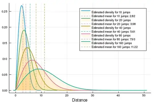
EDIT 2: adding some histograms that approximate the densities

enter image description here

For $n\le 5$ the estimated densities are strange (not of bell form), however for $n=2$ the density approaches the theoretical density, that is

$$f_{Y_2}(x)=\frac1{\pi\sqrt{1-(x/2)^2}}\chi_{[0,2]}(x)$$

(Note the vertical asymptote at $x=2$ in $f_{Y_2}$. Anyway the empirical approximation tends to it). If someone is interested this was the code, written in Julia, that I had used for the simulations:

# Sum of random jumps in the plane
function rsum(n::Int)
    p = 1.0
    for j in 2:n
        p += exp(2pi * im * rand())
    end
    return p
end

# Distance after n random jumps
function rd(n::Int)
    abs(rsum(n))
end

 # Data array to build an histogram
 function sim(n::Int, m::Int = 22)
    datos = zeros(2^m)
    for i in 1:2^m
        datos[i] = rd(n)
    end
    return datos
 end

# Plotting densities
using StatsPlots, Statistics
function dd(n::Int,m::Int=22)
    x = sim(n,m)
    density!(x, w = 2,
        xlabel = "Distance",
        label = "Estimated density for $n jumps",
        fill = (0, 0.1, :orange))
    vline!([mean(x)],
        label = "Estimated mean for $n jumps: $(round(mean(x),digits=2))",
        line = :dash)
end
Masacroso
  • 30,417
  • 2
    Hint: Central Limit Theorem – Robert Israel Jul 16 '19 at 14:57
  • @RobertIsrael Im not sure how to apply properly the central limit theorem in this context. – Masacroso Jul 16 '19 at 17:33
  • @Masacroso I think Robert Israel is right, assuming that $n$ is sufficiently big. – the_candyman Jul 16 '19 at 18:32
  • 1
    @the_candyman but, if Im not wrong, we have that $\sigma,\mu=0$ for each r.v. $e^{ i X_k}$, and as far as I know the normal distribution is not defined for $\sigma=0$ – Masacroso Jul 16 '19 at 18:42
  • 2
    @Masacroso: You are wrong :) The mean of $e^{i X_k}$ is zero but the standard deviation is 1. The mean of the sum is also zero, but the mean of its absolute value is not zero. – Nate Eldredge Jul 16 '19 at 18:57
  • @Masacroso I think that there is a "central limit theorem" dealing with the sum of the square of i.i.d. rv. In this case, I think that the limit pdf is Chi squared (as you already suspect). – the_candyman Jul 16 '19 at 19:01
  • @NateEldredge how you calculate $\sigma$? To me we have that $$\sigma^2(e^{ i X})=E[(e^{ i X}-\mu)^2]= E[e^{i 2X}]=\frac1{2\pi}\int_{-\pi}^\pi e^{i 2x} dx=\frac1{2\pi i}\oint z^2 dz=0$$ Where is my mistake? – Masacroso Jul 16 '19 at 19:15
  • 1
    The definition $\operatorname{Var}(Y) = E[(Y-\mu)^2]$ is only reasonable for real-valued random variables, not complex-valued. You really need a covariance matrix as in Robert's answer. But what I had in mind is that $E[|e^{i X_k}-\mu|^2] = 1$. – Nate Eldredge Jul 16 '19 at 19:18

1 Answers1

2

Since we'll be working with both real and imaginary parts, it's convenient to consider them as components of a vector: $$ V_k = [\cos(X_k), \sin(X_k)] $$ Note that these have mean $0$ and covariance matrix $$ \Sigma = \pmatrix{1/2 & 0\cr 0 & 1/2\cr}$$ By the multivariate version of the Central Limit Theorem, if $S_n = \sum_{k=1}^n V_k$, $ S_n/\sqrt{n} $ tends in distribution to a bivariate normal random variable with mean $0$ and covariance matrix $\Sigma$. In particular, the distribution of $|S_n|/\sqrt{n}$ approaches that of $\sqrt{(Z_1^2 + Z_2^2)/2}$ where $Z_1$ and $Z_2$ are independent standard normal random variables. It can be shown (by using polar coordinates) that this has PDF $2 r e^{-r^2}$ for $r > 0$.

Robert Israel
  • 448,999