I started a bounty on this question here: General point process - expected number of arrivals within an interval. The premise is that we have a point process where the time between successive events is a random variable $T$. The first moment of $T$ exists and is given by $E(T)=t$. And that's all we assume about $T$. Successive draws from it in the point process might even be correlated.
Now, we go to a random time, $J$ where we're going to start our observation window. It's important for $J$ to be such that it doesn't confer preferential treatment to any point of the point process. One way to achieve this is to have $J$ be uniform distributed over $(0,m)$ and take the limit $m \to \infty$.
I conjectured in the question above that if we take an interval of size $u$ starting at $J$ and count the number of events from the point process, the average number of events that fall into it will be:
$$E(N) = \frac{u}{t}$$.
At the very end of the question in the link above is a Python simulation where you can plug in various distributions for $T$ and verify that the conjecture continues to hold. I believe now that I have a proof for this. I need help validating this proof and see if there are any holes in it.
The proof
We can express $T=t+\epsilon$ where $E(\epsilon)=0$ by definition. We first consider the deterministic point process where $\epsilon=0$ and events simply happen every $t$ interval. We first show that the conjecture holds for this point process in case-2 of the question linked above. We will now try to transform the general point process into this case.
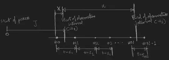
This is what our observation of the point process looks like. We go from the start of it to some time $J$ and take an interval of size $u$ starting there. The end of the observation interval is labeled $u_2$ and the start of it is labeled $u_1$.
We label the point lying just before our interval started "#$0$", the first point inside our observation window "#$1$" and so on until the last point in our observation window which is "#$N$" (so, we have $N$ points lying inside our observation window). The point lying just outside our observation window is "#$N+1$". The inter-arrival time between event #$i$ and #$i+1$ is $t+\epsilon_i$ where $t$ is the mean time between arrivals for our point process. Again, all we know about the $\epsilon_i$'s is that their means are $0$ and their domains are $(-t, \infty)$.
Now, we want to take convert this general point process to the deterministic one. Let's start with $\epsilon_1$. To remove this source of randomness from the point process, we simply consider an alternate point process which is identical to the one we're considering in every respect, apart from the fact that event #$2$ happened $t$ after event #$1$ and not $t+\epsilon_1$. We can achieve this by moving event #$2$ backwards in time by $\epsilon_1$. Note that this moves all events after event #$2$ back by this amount.
But now, there is a chance that the number of events in our interval will increase to more than $N$ since event #$N+1$ could be dragged into our interval. To keep this the same, we move $u_2$ back by $\epsilon_1$ as well. Repeating this for events #$3$ through #$N+1$, we have managed to make the inter-arrival times between events #$1$ through $N+1$ deterministic. But now we don't take an interval of size $u$, instead an interval of size $V=u-(\epsilon_1+\epsilon_2+\dots \epsilon_N)$. Note that we don't know anything about the $\epsilon$'s or how many there are, but we do know each of them has expected value $0$. In other words, $E(V)=u$. So, we can consider that we were dealing with the deterministic point process and took an interval of size $V$ instead of $u$ (which is stochastic now).
There is still one issue though. We haven't managed to remove $\epsilon_0$ in this same way. This is because moving the first event back by $\epsilon_0$ might cause event #$0$ to now fall inside our interval. And we don't want to move the start of the interval because we might lose the property that it doesn't confer "preferential treatment" on any of the points. So, we simply condition on $\epsilon_0$.
Per the figure above, the random variable denoting the time between the start of the interval and the occurrence of event #$1$ is $X$. We count the first event and the time in our interval left after it is $V-X$ (in the modified point process). And we have established that event #$2$ happens $t$ after event #$1$ and so on. So, the number of events inside our interval in the modified point process becomes:
$$N = 1+\left[\frac{V-X}{t}\right] = 1+\left[\frac{u-\epsilon_s-X}{t}\right]$$
Here, $[x]$ is the greatest integer less than or equal to $x$, $\epsilon_s = \epsilon_1+\epsilon_2+\dots +\epsilon_N$ and conditional on $\epsilon_0$, $X$ is uniformly distributed between $(0, t+\epsilon_0)$. We can then say:
$$N=1+\left[\frac{u}{t}-\frac{\epsilon_s}{t}-\left(1+\frac{\epsilon_0}{t}\right) U\right] = 1+\left[\frac{u}{t}-\frac{\epsilon_s}{t}-\left(1+\frac{\epsilon_0}{t}\right) U\right]$$
$$=1+\left[\frac{u}{t}-\left(\frac{\epsilon_s}{t}+\frac{\epsilon_0}{t}U \right)- U\right]=1+\left[\frac{u}{t} + \eta -U\right]$$
where $U$ is uniformly distributed between $(0,1)$ and $\eta$ is a random variable with mean $0$.
Taking expectation on both sides and using the fact that $E([c+\eta-U])=c-1$ when $\eta$ has mean $0$ we get the desired result.
$$E(N) = \frac{u}{t}$$
For the fact that $E([c+\eta-U])=c-1$ which we used above, here is a proof for the case where $\eta=0$: Prove that $E([c-U]) = c-1$ and its very easy to extend to the case where $\eta$ is a random variable with mean $0$ by conditioning on it.

