1

I have written a code like follows:

 TD1 = 200
    Debye1[T_] := 3 (T/TD1)^3 NIntegrate[y^3/(Exp[y] - 1), {y, 0, TD1/T}]
    Fa1[T_] := 8.6173324*10^(-5) T (9 *TD1/(8 T) + 
        3 Log[1 - Exp[-TD1/T]] - Debye1[T])


    TD2 = 300
    Debye2[T_] := 3 (T/TD2)^3 NIntegrate[y^3/(Exp[y] - 1), {y, 0, TD2/T}]
    Fa2[T_] := 8.6173324*10^(-5) T (9 *TD2/(8 T) + 
        3 Log[1 - Exp[-TD2/T]] - Debye2[T])

    DF[T_] := Fa2[T] - Fa1[T] + 0.037
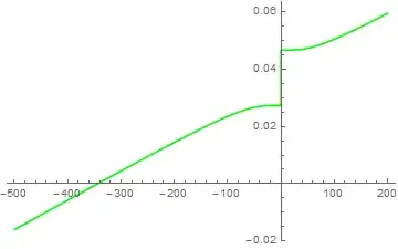
    Plot[DF[T], {T, 0, 500}, PlotStyle -> Green]

The plot looks like this: enter image description here

Upto this it works. But I am interested in the intersection point. So then I used the following:

Solve[DF[T]==0,T]

I am expecting something around ~100. Why am I not getting this? Is it something wrong with the Solve syntax?

The error I am getting like this:

NIntegrate::nlim: "y = 300./T is not a valid limit of integration."
General::stop: "Further output of NIntegrate::nlim will be suppressed during this calculation"
Solve::inex: Solve was unable to solve the system with inexact coefficients or the system obtained by direct rationalization of inexact numbers present in the system. Since many of the methods used by Solve require exact input, providing Solve with an exact version of the system may help.

Since I am quite new in Mathematica, any suggestion would be great help.

J. M.'s missing motivation
  • 124,525
  • 11
  • 401
  • 574
baban
  • 141
  • 8
  • 2
    Use FindRoot[] instead of Solve[]. Note that the Debye function can be represented in terms of special functions known to Mathematica, so the NIntegrate[] is not really needed here. – J. M.'s missing motivation Feb 16 '16 at 19:24
  • @J.M.: Yes, I have tried FindRoot, still it does not work. I know that Debye function is defined in Mathematica, but I wanted to define it in my way which works perfectly, but somehow it does not work in this particular case. – baban Feb 16 '16 at 19:29
  • 1
    "still it does not work" - can you post the code you've tried? You already have a good guess from your plot, which you can then feed into FindRoot[]. – J. M.'s missing motivation Feb 16 '16 at 19:32
  • I tried this: FindRoot[DF[T] == 0, {T, 0}]. But it shows: FindRoot::nlnum: "The function value {Indeterminate} is not a list of numbers with dimensions {1} at {T} = {0.`}." Infinity::indet: "Indeterminate expression E^ComplexInfinity encountered. "

    If I use this: FindRoot[DF[T] == 0, T] then it shows: FindRoot::fdss: Search specification T should be a list with 1 to 5 elements.

    – baban Feb 16 '16 at 19:35
  • You provided a bad guess, even when you already have a good one. 0 is quite far away from 100, so I'm not surprised. Try FindRoot[DF[T] == 0, {T, 100}]. – J. M.'s missing motivation Feb 16 '16 at 19:39
  • Still it does not work. Whatever the value I am giving in the parenthesis after T it shows that one. E.g., FindRoot[DF[T] == 0, {T, 100}] and FindRoot[DF[T] == 0, {T, 50}] gives value T->100. and T->50. respectively with the following message: FindRoot::njnum: "The Jacobian is not a matrix of numbers at {T} = {100.}" NIntegrate::vars: Integration range specification Compile$54 is not of the form {x, xmin, ..., xmax}. – baban Feb 16 '16 at 19:45
  • Your question may be put on-hold as it seems to be off-topic, i.e it arises from a simple mistake and is unlikely to help any future visitors. Don't be discouraged by that cleaning-up policy. Your future good questions are welcome. Learn about common pitfalls here. – rhermans Feb 16 '16 at 20:08
  • Your function never gets near zero: Plot[DF[T], {T, 0, 500}, PlotStyle -> Green, PlotRange -> {{0, 0.1}}] – Mr.Wizard Feb 16 '16 at 23:30

3 Answers3

4

You have to be careful where Plot positions your axes; in your original plot the point where the green line crosses the axis corresponds to an ordinate of ca. 0.05, NOT zero.

To see the situation more clearly, expand your plot range, and force the axes origin to be at $(0,0)$:

Plot[DF[T], {T, -500, 200}, PlotStyle -> Green, PlotRange -> All, AxesOrigin -> {0, 0}]

Mathematica graphics

You will notice that your zero crossing actually happens at negative values of T, around -350.

You can use FindRoot to find that precisely:

FindRoot[DF[T], {T, -350}]

Although this returns a correct answer, it also returns complaints from the NIntegrate embedded in your definition of the Debye function because it attempts to evaluate the function symbolically before it is passed numerical values. Prevent non-numerical evaluation by re-defining DF to only evaluate when explicitly numerical input is given using NumericQ:

Clear[DF]
DF[T_?NumericQ] := Fa2[T] - Fa1[T] + 0.037
FindRoot[DF[T], {T, -350}]

(* Out: {T -> -344.081 + 0. I} *)

This returns a vanishingly small imaginary part to your solution, which should not be there and is probably caused by rounding error, so force the use of arbitrary precision numbers instead:

FindRoot[DF[T], {T, -350}, WorkingPrecision -> $MachinePrecision]

(* Out: {T -> -344.0814892394558} *)

This uses arbitrary precision calculations with the same number of precision digits as a normal machine precision number. Crucially, however, using arbitrary precision allows for precision tracking of the result, which in turns allows the system to remove the small imaginary part caused by inexact calculations.

MarcoB
  • 67,153
  • 18
  • 91
  • 189
2

I have solved your functions with Integrate. The result is the same as MarcoB's.

TD1 = 200
Debye1[T_] = 3 (T/TD1)^3 Integrate[y^3/(Exp[y] - 1), {y, 0, TD1/T}, Assumptions -> T > 0];
Fa1[T_] = Rationalize[8.6173324*10^(-5) T (9*TD1/(8 T) + 3 Log[1 - Exp[-TD1/T]] - Debye1[T]), 0]

(* (1/3895544287)335692 T (225/T + 3 Log[1 - E^(-200/T)] - (1/8000000)
   3 T^3 (-(\[Pi]^4/15) - 400000000/T^4 + (8000000 I \[Pi])/T^3 + (
      8000000 Log[-1 + E^(200/T)])/T^3 + (
      120000 PolyLog[2, E^(200/T)])/T^2 - (
      1200 PolyLog[3, E^(200/T)])/T + 6 PolyLog[4, E^(200/T)])) *)

TD2 = 300
Debye2[T_] = 3 (T/TD2)^3 Integrate[y^3/(Exp[y] - 1), {y, 0, TD2/T}, Assumptions -> T > 0];
Fa2[T_] = Rationalize[8.6173324*10^(-5) T (9*TD2/(8 T) + 3 Log[1 - Exp[-TD2/T]] - Debye2[T]), 0]

(*(1/3895544287)335692 T (675/(2 T) + 3 Log[1 - E^(-300/T)] - (1/
   9000000)T^3 (-(\[Pi]^4/15) - 2025000000/T^4 + (27000000 I \[Pi])/
      T^3 + (27000000 Log[-1 + E^(300/T)])/T^3 + (
      270000 PolyLog[2, E^(300/T)])/T^2 - (
      1800 PolyLog[3, E^(300/T)])/T + 6 PolyLog[4, E^(300/T)])) *)

DF[T_] = Fa2[T] - Fa1[T] + Rationalize[0.037, 0] // FullSimplify

(* (55910894927130000 - 1594537 \[Pi]^4 T^4 + 
   271910520000000 T (Log[1 - E^(-300/T)] - Log[1 - E^(-200/T)] + 
      Log[-1 + E^(200/T)] - Log[-1 + E^(300/T)]) + 
   7553070 T^2 (540000 PolyLog[2, E^(200/T)] - 
      360000 PolyLog[2, E^(300/T)] + 
      T (-5400 PolyLog[3, E^(200/T)] + 2400 PolyLog[3, E^(300/T)] + 
         27 T PolyLog[4, E^(200/T)] - 
         8 T PolyLog[4, E^(300/T)])))/1051796957490000000 *)

Plot[DF[T], {T, -500, 100}, PlotStyle -> Green, PlotPoints -> 100]

enter image description here

FindRoot[DF[T] == 0, {T, -300}]

(* {T -> -344.081 + 0. I} *)
  • Thank you so much, actually there was a typo in my code (extremely sorry for that) so the answer I was looking for around 344. You got the trick, thanks! That's solved my problem. – baban Feb 17 '16 at 09:55
  • +1, but Assumptions -> T > 0 when the solution is T -> -344.081? May be enough with Assumptions ->Element[T,Reals] – rhermans Feb 17 '16 at 09:59
  • @ rhermans Thanks for the hint. The specified functions are a contradiction in terms. My answer should indicate that ( Assumptions -> T > 0 and the plot T < 0). The code snippet Integrate[y^3/(Exp[y] - 1), {y, 0, TD1/T}, Assumptions -> T > 0] is o.k. –  Feb 17 '16 at 16:06
  • @rhermans If you set Assumptions ->Element[T,Reals] you get a ConditionalExpression with T < 0. The integral should therefore be Integrate[y^3/(Exp[y] - 1), {y, TD1/T, 0}, Assumptions -> T < 0]. The OP has recognized that it is a typo in his code and thus helped him, I hope so. –  Feb 17 '16 at 16:07
1

Your function does not cross zero around 100, so no surprize Mathematica can't find a solution around there.

Plot[DF[T], {T, -100, 100}, PlotStyle -> Green, PlotRange -> {0, 0.1}]

Mathematica graphics

I would say that you function crosses the $Y$ axis around 0.0467 on the rhs and 0.0273 on th lhs.

Chop[DF /@ {0.01, -0.01}]

{0.0466945, 0.0273055}

rhermans
  • 36,518
  • 4
  • 57
  • 149
  • @rhermas: Thanks, but what should I do then as an alternative to find that cross point in my plot, if I don't have guess? Any idea please? – baban Feb 16 '16 at 19:54
  • There is something missing. The value of the function is initially negative for small T and then it goes positive for large T (in my original plot). So, there should be only one value. I am interested in the positive value of T. I am looking for a simple crossing point of DF[T] for a T. – baban Feb 16 '16 at 20:11
  • @baban No, the function value is NOT initially negative in your first plot: it is positive throughout; you are being tricked by the positioning of the axes. Look at the values on your $y$ axis. If you want to see if more clearly, try Plot[DF[T], {T, -500, 200}, PlotRange -> All, AxesOrigin -> {0, 0}]. Your actual zero-crossing point is around $T=-344$. – MarcoB Feb 16 '16 at 20:36
  • @MarcoB: Thanks, that's what I was looking for. There was some typo in my script but nevertheless it would be 344. – baban Feb 17 '16 at 09:53