In a ListPlot of LinearModelFit, Fill to the regression line

Question

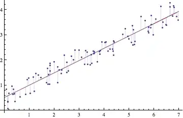
In the help for LinearModelFit, the regression line can be added to the scatter plot like this:

Show[ListPlot[data], Plot[lm[x], {x, 0, 5}]]

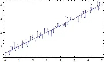
Is it possible to fill from the points to the regression line? This can illustrate the distance whose sum of squares is being minimized. I tried variations on this:

Filling -> Table[ lm[data[[i]][[2]]],  {i, Length[data]}]]

Here the Table will be a list of predicted values for y at each observation of x, but this results in the error "not a valid filling specification."

VLC · Accepted Answer · 2012-09-30T17:19:28.187

17

Maybe something like this:

data = Table[{x, .5 + .5 x + RandomReal[{-.5, .5}]}, {x, 
    RandomReal[7, 100]}];
lm = LinearModelFit[data, x, x];
ListPlot[{data, Table[{x,lm[x]}, {x, 0, 7, .1}]}, Joined -> {False, True}, 
    Filling -> 1 -> {2}]

enter image description here

edited Sep 30 '12 at 17:19

answered Sep 30 '12 at 16:54

VLC

9,818
1
31
60

Dr. belisarius · Answer 2 · 2012-10-01T08:22:08.447

9

Another way, using the properties of LinearModelFit, and a convoluted way for constructing lines (note that all the plot is done with only one ListLinePlot)

verba = Table[{x, .5 + .5 x + RandomReal[{-.5, .5}]}, {x, RandomReal[7, 100]}];
lm = LinearModelFit[verba, x, x];
res = Transpose@{verba[[All, 1]], lm["PredictedResponse"]};
ListLinePlot[Flatten[Transpose@{res, verba, res}, 1], Mesh -> All, Frame -> True]

Mathematica graphics

edited Oct 01 '12 at 08:22

answered Sep 30 '12 at 21:58

Dr. belisarius

115,881
13
203
453

(+1) could also use lm["PredictedResponse"] instead of #[[2]] - lm["FitResiduals"] when defining res. – kglr Sep 30 '12 at 22:13
@kguler thanks! Edited. – Dr. belisarius Sep 30 '12 at 22:23

score 8 · Answer 3 · answered Sep 30 '12 at 18:01

Another possibility, using ErrorBar :

Needs["ErrorBarPlots`"]

data = Table[{x, .5 + .5 x + RandomReal[{-.5, .5}]}, {x, 
RandomReal[{-5, 5}, 20]}];lm = LinearModelFit[data, x, x];

dataAndError = {#, ErrorBar[(-#[[2]] + lm[#[[1]]]) {Boole[#[[2]] >= lm[# [[1]]]] , Boole[#[[2]] < lm[#[[1]]]] }]} & /@ data;

Show[Plot[lm[x], {x, -5, 5}, PlotStyle -> {Red}], ErrorListPlot[dataAndError]]

plot

Alexei Boulbitch · Answer 4 · 2012-10-01T12:14:45.823

3

One may simply draw them as follows. This is the list of data:

lst = Table[{i, 0.5 + 0.5*i^(1/2) + RandomReal[{-.5, .5}]}, {i, 1, 10}]

This is the fitting:

ft = FindFit[lst, a*x^(1/2) + b, {{a, 0.4}, b}, x]

And this draws the fitting function together with the list and draws lines from the points specified by the list to the curve:

f[x_] := a*x^(1/2) + b /. ft
lst1 = Transpose[lst][[1]];

Show[{ListPlot[lst, PlotStyle -> Red], Plot[f[x] /. ft, {x, 0, 10}],


Graphics[   
     {Pink, Line[Transpose[{lst, Transpose[{lst1, Map[f, lst1]}]
                                              }]]} ]}]

That is the outcome: enter image description here

edited Oct 01 '12 at 12:14

answered Oct 01 '12 at 12:10

Alexei Boulbitch

39,397
2
47
96

2

lst1 = Transpose[lst][[1]]; can also be done this way: lst1 = lst[[All, 1]]; – J. M.'s missing motivation Oct 01 '12 at 12:18

score 2 · Answer 5 · answered Oct 01 '12 at 08:41

Yet another possibility, using Arrow[]+Arrowheads[]:

(* for reproducibility *)
BlockRandom[SeedRandom[42, Method -> "Legacy"];
            data = Sort[Table[{x, .5 + .5 x + RandomVariate[NormalDistribution[]]/5},
                              {x, RandomReal[7, 100]}]]];

lm = LinearModelFit[data, x, x];

Show[Graphics[{ColorData[1, 1], 
               Arrowheads[{{Automatic, Automatic, Graphics[Point[{0, 0}]]}}], 
               MapThread[Arrow[{##}] &,
                         {Transpose[{data[[All, 1]], lm["PredictedResponse"]}], data}]}],
     Plot[lm[x], {x, 0, 7}], Frame -> True]

regression line and data points

In a ListPlot of LinearModelFit, Fill to the regression line

5 Answers5

Linked