We can use ifnToBezierCurve[] from Convert interpolating function to a Bezier curve, which I converted to a package.
Proof of concept
The following shows a very minimal example. I limited the number of points plotted. I also used Show[] to remove the axes so that the ExportString[] would not have compressed data.
Get@"https://raw.githubusercontent.com/mroge02/ifnToBezierCurve/main/ifnToBezierCurve.wl"
plot = Plot[x^3 - 2 x^2, {x, 0, 2}, PlotPoints -> 4,
   MaxRecursion -> 0];
bezierPlot = Normal@Show[plot, Axes -> None] /.
   Line[p_] :> ifnToBezierCurve@Interpolation[p];
ExportString[bezierPlot, "EPS"]
%!PS-Adobe-3.0 EPSF-3.0
...
%%BeginProlog
...
/c { curveto } bind def
...
%%EndProlog
...
0.368414 0.506783 0.709804 rg
1.44 w
2 J
0 j
[] 0.0 d
3.25 M 5.184 8.008 m 31.777 8.012 58.367 41.352 84.961 75.969 c 113.789 113.5
142.617 152.523 171.445 152.184 c 198.969 151.859 226.492 115.656 254.016
 8.012 c S
Q Q
showpage
%%Trailer
end
%%EOF
Visualization.
The following shows the original plot and a comparison of the Bezier curve plot the regular plot of the function. Because the number of points is very small, the Plot[] polyline does not reflect the curvature of the graph, whereas the cubic Bezier curve draws the graph of the cubic exactly.
GraphicsRow[{plot /.
   Line[p_] :> {Line[p], Directive[Magenta, PointSize@Large],
     Point[temp = p]},
  Show[
   Plot[x^3 - 2 x^2, {x, 0, 2},
    PlotStyle -> {AbsoluteThickness[6], Black}],
   Plot[x^3 - 2 x^2, {x, 0, 2},
    PlotStyle -> {AbsoluteThickness[5], LightYellow}],
   bezierPlot,
   Graphics[{Directive[Magenta, PointSize@Large], Point[temp]}],
   Axes -> True]
  }]

A more robust replacement rule
Another example with a normal plot, which also shows how to process a line in a GraphicsComplex.
lineToBezier = {
   GraphicsComplex[pts_, g_, opts___] :>
    GraphicsComplex[pts,
     g /. {Line[p_?(VectorQ[#, IntegerQ] &)] :>
        ifnToBezierCurve@Interpolation[pts[[p]]]}, opts],
   Line[p_?(MatrixQ[#, Developer`RealQ] &)] :>
    ifnToBezierCurve@Interpolation[p]
   };
Plot[Sin[x], {x, 0, 2 Pi}, Mesh -> 15,
  MeshStyle -> Red] /. lineToBezier
Note that converting to Bezier curves would destroy any gradient coloring of the curve. (Line supports VertexColors, but BezierCurve does not in 2D.)
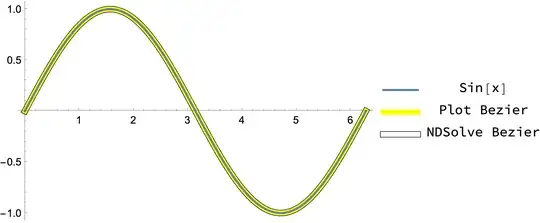
Using NDSolve to avoid oversampling
Plot generates a lot of points. If you want fewer points, using NDSolve is perhaps a more efficient approach.
plot2 = Plot[Sin[x], {x, 0, 2 Pi}];
{ifn1} = Cases[
   plot2,
   Line[p_] :> Interpolation[p],
   Infinity];
ifn2 = NDSolveValue[{y'[x] == D[Sin[x], x], y[0] == Sin[0]},
   y, {x, 0, 2 Pi},
   (* pick order/precision appropriate for a plot *)
   Method -> {"ExplicitRungeKutta", "DifferenceOrder" -> 3},
   PrecisionGoal -> 3];
Comap[{ifn1, ifn2}, "Grid"] // Map@Length
(* {431, 30} -- NDSolve has a lot fewer points *)
Visualization:
Labeled[
 Show[
  Graphics[{
    Black,
    AbsoluteThickness[6],
    ifnToBezierCurve[ifn1],
    Yellow,
    AbsoluteThickness[5],
    ifnToBezierCurve[ifn2]
    }, Options@Plot],
  plot2
  ],
 Grid[{{Graphics[{#[[1]] &[
       "DefaultPlotStyle" /. (Method /.
          Charting`ResolvePlotTheme[Automatic, Plot])],
      AbsoluteThickness[2], Line[{{0, 0}, {1, 0}}]},
     PlotRange -> {{-0.1, 1.1}, {-0.1, 0.1}}, ImageSize -> {40, 16}],
    HoldForm[Sin[x]]},
   {Graphics[{
      Yellow,
      AbsoluteThickness[5],
      Line[{{0, 0}, {1, 0}}]},
     PlotRange -> {{-0.1, 1.1}, {-0.1, 0.1}}, ImageSize -> {40, 16}]
    , "Plot Bezier"},
   {Graphics[{Black,
      AbsoluteThickness[6],
      Line[{{0, 0}, {1, 0}}],
      White,
      AbsoluteThickness[5],
      Line[{{0, 0}, {1, 0}}]},
     PlotRange -> {{-0.1, 1.1}, {-0.1, 0.1}}, ImageSize -> {40, 16}]
    , "NDSolve Bezier"}}],
 Right
 ]


Plot[]produces a polyline and not a Bézier curve. You'll have to do more work if you absolutely must have a Bézier. – J. M.'s missing motivation Jul 07 '16 at 12:39