35

Given a set of data, is it possible to create a linear regression which has a slope error that takes into account the uncertainty of the data?

This is for a high school class, and so the normal approach to find the uncertainty of the slope of the linear regression is to find the line that passes through the first data point minus its uncertainty and the last data point plus its uncertainty, and vice versa. Then, the slope of the line with the greater slope is subtracted from the other slope. However, this is not very accurate. Is there another way?

Both the x-coordinate and y-coordinate has an associated error. However, the error in the x-coordinate can be safely ignored without loss of marks. I would prefer a solution that takes into account both errors, but one that takes into account only the error in the y-coordinate is acceptable.

George S
  • 353
  • 1
  • 4
  • 5
  • Welcome to Mathematica.SE! Can you please confirm that you plan to do this analysis in Mathematica? Otherwise I think it would be better to migrate your question to Cross Validated. – Verbeia Oct 15 '12 at 00:55
  • 6
    It is commendable that you plan on using Mathematica for a high school project/class. – dearN Oct 15 '12 at 00:56
  • @Verbeia: Hi, yes, I plan on doing this all in Mathematica. and drN, Thank you! – George S Oct 15 '12 at 01:03
  • @drN I think it's commendable that they are running regressions in high school! – Verbeia Oct 15 '12 at 01:40
  • 1
    These might be relevant: http://onlinelibrary.wiley.com/doi/10.1002/aic.10540/abstract and http://www.physicsforums.com/showthread.php?t=156642 – s0rce Oct 15 '12 at 01:53
  • If I understand you correctly, your data is of the form $(x_k,y_k,\sigma_k)$, where $(x_k,y_k)$ is a data point, and $\sigma_k$ is the associated uncertainty (meaning your $y_k$ is actually the interval $y_k\pm\sigma_k$)? – J. M.'s missing motivation Oct 15 '12 at 01:56
  • 2
    @J.M. Almost, there is an additional uncertainty on the x variable, so $(x_k, y_k, \text{xerr}_k, \text{yerr}_k)$, becoming $(x_k \pm \text{xerr}_k, y_k \pm \text{yerr}_k)$. – George S Oct 15 '12 at 02:13
  • @s0rce I am unable to access the paper.

    The most helpful equation in the thread on physicsforums "sigma(slope) = |slope| tan[arccos(R)]/sqr(N-2)" does not seem to take into account uncertainty at all, unless the correlation coefficient R does this somehow?

    In addition, I am unsure about the meaning of the function "sqr" and how many degrees of freedom my data has.

    – George S Oct 15 '12 at 02:23
  • 1
    @George, that is a very important piece of detail. Please edit your question to mention that both your abscissas and ordinates have associated errors. – J. M.'s missing motivation Oct 15 '12 at 02:35
  • @J.M. done, although the error in the x-coordinate can be ignored if that is required. – George S Oct 15 '12 at 02:39
  • 1
    I'm not saying it's required; you're the only one who is supposed to determine whether they should be accounted for or ignored. My point was that weighted orthogonal regression (which accounts for errors in both coordinates) is a tougher problem to solve (and thus requires more elaborate methods) than weighted linear regression, which is easily handled by the built-in function LinearModelFit[] (via its Weights option). – J. M.'s missing motivation Oct 15 '12 at 02:52
  • The same issue has just arisen on Cross Validated at http://stats.stackexchange.com/questions/40453. – whuber Oct 15 '12 at 15:12
  • @GeorgeS What level of complexity would you like to expose your students to ? – image_doctor Oct 15 '12 at 17:05
  • @image_doctor It's the other way around. : P I'm a student doing a physics lab write-up. I used Mathematica for a mathematics project and found it very useful, and want to use it in my write-up as well. – George S Oct 15 '12 at 22:33
  • @GeorgeS sorry my mistake, I misunderstood, congratulations on your perspicacity! – image_doctor Oct 16 '12 at 07:16
  • 1
    The Matlab code for this problem can be found at https://de.mathworks.com/matlabcentral/fileexchange/17466-weighted-total-least-squares-straight-line-fit https://de.mathworks.com/matlabcentral/fileexchange/30193-weighted-total-least-squares-for-mutually-correlated-coordinates Maybe this helps. – M. Krystek Feb 18 '17 at 09:27
  • @M.Krystek Thanks for sharing this. Link only answers are discouraged so I converted your post into a comment. I know that you do not have enough "reputation" points to post a comment yet. (An anti-spam measure I believe.) – Mr.Wizard Feb 18 '17 at 10:31

6 Answers6

28

Here's a method for doing weighted orthogonal regression of a straight line, based on the formulae in Krystek/Anton and York:

ortlinfit[data_?MatrixQ, errs_?MatrixQ] := 
 Module[{n = Length[data], c, ct, dk, dm, k, m, p, s, st, ul, vl, w, wt, xm, ym},
        (* yes, I know I could have used FindFit[] for this... *)
        {ct, st, k} = Flatten[MapAt[Normalize[{1, #}] &, 
           NArgMin[Norm[Function[{x, y}, y - \[FormalM] x - \[FormalK]] @@@ data],
                   {\[FormalM], \[FormalK]}], 1]];
        (* find orthogonal regression coefficients *)
        {c, s, p} = FindArgMin[{
           Total[(data.{-\[FormalS], \[FormalC]} -
                 \[FormalP])^2/((errs^2).{\[FormalS]^2, \[FormalC]^2})],
           \[FormalC]^2 + \[FormalS]^2 == 1},
          {{\[FormalC], ct}, {\[FormalS], st}, {\[FormalP], k/ct}}];
        (* slope and intercept *)
        {m, k} = {s, p}/c;
        wt = 1/errs^2; w = (Times @@@ wt)/(wt.{1, m^2});
        {xm, ym} = w.data/Total[w];
        ul = data[[All, 1]] - xm; vl = data[[All, 2]] - ym;
        (* uncertainties in slope and intercept *)
        dm = w.(m ul - vl)^2/w.ul^2/(n - 2);
        dk = dm (w.data[[All, 1]]^2/Total[w]);
        {Function[\[FormalX], Evaluate[{m, k}.{\[FormalX], 1}]], Sqrt[{dm, dk}]}] /;
     Dimensions[data] === Dimensions[errs]

ortlinfit[] expects data to contain the $(x_j,y_j)$ pairs, and errs to contain the corresponding uncertainties $(\rm{dx}_j,\rm{dy}_j)$. The routine returns the best-fit line as a pure function, as well as the uncertainties in the slope and intercept ($\sigma_m$ and $\sigma_k$).

As an example, here's some data used in York's paper:

data = {{0, 5.9}, {0.9, 5.4}, {1.8, 4.4}, {2.6, 4.6}, {3.3, 3.5}, {4.4, 3.7},
        {5.2, 2.8}, {6.1, 2.8}, {6.5, 2.4}, {7.4, 1.5}};

errs = {{1000., 1.}, {1000., 1.8}, {500., 4.}, {800., 8.}, {200., 20.},
        {80., 20.}, {60., 70.}, {20., 70.}, {1.8, 100.}, {1, 500.}} // Sqrt[1/#] &;

{lin, {sm, sk}} = ortlinfit[data, errs]
   {Function[x, 5.47991 - 0.480533 x], {0.0710065, 0.361871}}

Now, let's look at the data, the associated error ellipses (constructed from the uncertainties), the best-fit line, and the "bounding lines" $(m-\sigma_m)x+(k-\sigma_k)$ and $(m+\sigma_m)x+(k+\sigma_k)$:

Show[
     Graphics[{AbsolutePointSize[4], Point[data], MapThread[Circle, {data, errs}]},
              Frame -> True], 
     Plot[{lin[x], lin[x] - sm x - sk, lin[x] + sm x + sk}, {x, -1, 9},
          PlotStyle -> {Directive[Thick, Red],
                        Directive[Dashed, Gray], Directive[Dashed, Gray]}]
     ]

plot of best-fit line with errors in both coordinates

J. M.'s missing motivation
  • 124,525
  • 11
  • 401
  • 574
  • At the bottom of your example you call the function with an undefined wts (presumably errs); also I get a different output : {Function[\[FormalX]$, 5.76267 - 0.536842 \[FormalX]$], {0.0468427, 0.198548}}. My approach gives a not too bad solution : {a -> -0.539577, b -> 5.76119} for the parameters and {0.0609037, 0.206709} for their errors. – b.gates.you.know.what Oct 16 '12 at 08:17
  • Whoops, thanks for catching that typo! (That was from a previous test, which I forgot to fix here.) Please try the code now. – J. M.'s missing motivation Oct 16 '12 at 08:48
  • 1
    A big +1. Now you got me wondering, how this problem could be solved for arbitrary curves (so for non-linear regression) – Ajasja Oct 16 '12 at 09:48
  • 1
    @Ajasja:: the unweighted case of nonlinear orthogonal regression is already a bit difficult; more so if we have to account for weights/uncertainties. I'd say that should be for a different question... :) (However, the algorithm for unweighted orthogonal regression of a straight line is much simpler than the one I gave here; all that's needed is a clever application of the SVD.) – J. M.'s missing motivation Oct 16 '12 at 09:55
  • When y data is large I can't get it to find a fit. Here's some test data with all the weights set to 1. With 10^7 it finds a fit, with 10^8 it doesn't. Compared to LinearModelFit it appears that the y intercept is getting a progressively larger error. lm = LinearModelFit[data, x, x] Show[{ListPlot[data], Plot[lm[x], {x, 0, 10}]}] data = Transpose[{Range[10], 10^7 Range[10]}]; errs = ConstantArray[1, {10, 2}]; Show[{ListPlot[data], Plot[lin[x], {x, 0, 10}]}] I tried adjusting the options to FindArgMin but without success. What am I doing wrong? – DrBubbles Jun 29 '14 at 21:10
  • Ahh.. indeed ortlinfit[data, 10000 errs] is slightly different from ortlinfit[data, errs], but why ortlinfit is so insensitive to errors of x and y? – Harry Feb 29 '16 at 12:52
  • the error by ortlinfit is much smaller than errors by LinearModelFit[data, x, x]["ParameterErrors"]... – Harry Feb 29 '16 at 12:56
  • I found that ortlinfit seems have trouble on error estimation: ortlinfit[data, 100*errs] returns same result of ortlinfit[data,errs] !!! @J.M. – Harry Feb 29 '16 at 14:25
  • @Harry, what data and errs are you using? Are your errs actual uncertainties, or did you mean to use weights instead? – J. M.'s missing motivation Feb 29 '16 at 14:33
  • I use exactly the very same data and errs in your answer, which is: data = {{0, 5.9}, {0.9, 5.4}, {1.8, 4.4}, {2.6, 4.6}, {3.3, 3.5}, {4.4, 3.7}, {5.2, 2.8}, {6.1, 2.8}, {6.5, 2.4}, {7.4, 1.5}};

    errs = {{1000., 1.}, {1000., 1.8}, {500., 4.}, {800., 8.}, {200., 20.}, {80., 20.}, {60., 70.}, {20., 70.}, {1.8, 100.}, {1, 500.}} // Sqrt[1/#] &; then ortlinfit[data, 100*errs] returns almost same result of ortlinfit[data,errs] @J.M.

    – Harry Mar 01 '16 at 04:18
  • You mentioned that one could have used FindFit for that. In which cases this approach will be equivalent to that of FindFit? Also, how would one use orthogonal distance regression in FindFit? – mikeonly Oct 09 '16 at 11:20
  • @mike, the comment was referring to the line where {ct, st, k} was computed; if you look closely, it is just doing a classical least-squares fit, but rearranged slightly so that the required sine, cosine, and intercept are obtained directly. The rest of the routine, AFAICT, is not possible with FindFit[]. – J. M.'s missing motivation Oct 09 '16 at 11:24
  • @J.M., oh right, didn't realized that! Your code worked much better than built-in functions for a linear model I had. Thank you. – mikeonly Oct 09 '16 at 11:33
19

Summary

Use the Weights option to LinearModelFit, setting the weights to be inversely proportional to the variances of the error terms.


Theory

This is a standard problem: when the errors in the individual $y$ values are expressed in a way that can be related to their variances, then use weighted least squares with the reciprocal variances as the weights. (Search our sister site Cross Validated for more about this, including references and generalizations.)

Creating realistic data to study

To illustrate, suppose the data are given as vectors $x$ and $y$ with the "errors" expressed either as standard deviations of $y$ or as standard errors of estimate of $y$, or any other quantity that can be interpreted as a fixed, constant multiple of the standard deviations of the $y$. Specifically, the applicable model for these data is

$$y_i = \beta_0 + \beta_1 x_i + \varepsilon_i$$

where $\beta_0$ (the intercept) and $\beta_1$ (the slope) are constants to be estimated, the $\varepsilon_i$ are independent random deviations with mean zero, and $\text{Var}(\varepsilon_i) = \sigma_i^2$ for some given quantities $\sigma_i$ assumed to be known accurately. (The case where all the $\sigma_i$ equal a common unknown constant is the usual linear regression setting.)

In Mathematica we can simulate such data with random number generation. Let's wrap this into a function whose arguments are the amount of data and the slope and intercept. I will make the sizes of the errors vary randomly, but generally they will increase as $x$ increases.

simulate[n_Integer, intercept_: 0, slope_: 0] /; n >= 1 := 
 Module[{x, y, errors, sim},
  x = Range[n];
  errors = RandomReal[GammaDistribution[n, #/(10 n)]] & /@ x;
  y = RandomReal[NormalDistribution[intercept + slope  x[[#]],  errors[[#]]]] & / Range[n];
  sim["x"] = x;
  sim["y"] = y;
  sim["errors"] = errors;
  sim
  ]

Here is a tiny example of its use.

SeedRandom[17];
{x, y, errors} = simulate[16, 50, -2/3][#] & /@ {"x", "y", "errors"};
ListPlot[{y, y + errors, y - errors}, Joined -> {False, True, True}, 
 PlotStyle -> {PointSize[0.015], Thick, Thick}, 
 AxesOrigin -> {0, Min[y - errors]}]

Scatterplot

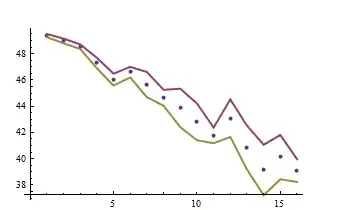
The simulated points are surrounded by error bands.

Weighted least-squares estimation

To fit these data, use the Weights option of LinearModelFit. Once again, let's prepare for later analysis by encapsulating the fitting in a function. For comparison, let's fit the data both with and without the weights.

trial[n_Integer: 1, intercept_: 0, slope_: 0] := 
 Module[{x, y, errors, t, fit, fit0},
  {x, y, errors} = simulate[n, intercept, slope][#] & /@ {"x", "y", "errors"};
  fit = LinearModelFit[y, t, t, Weights -> 1 / errors^2];
  fit0 = LinearModelFit[y, t, t];
  {fit[#], fit0[#]} & @ "BestFitParameters"
  ]

The output is a list whose elements give {intercept, slope}: the first element is for the weighted fit, the second for the unweighted.

Monte-Carlo comparison of the weighted and ordinary least squares methods

Let's run a lot of independent trials (say, $1000$ of them for simulated datasets of $n=32$ points each) and compare their results:

SeedRandom[17];
simulation = ParallelTable[trial[32, 20, -1/2], {i, 1, 1000}];

ranges = {{18.5, 22}, {-0.65, -0.35}};
TableForm[
  Table[Histogram[simulation[[All, i, j]], ImageSize -> 250, 
          PlotRange -> {ranges[[j]], Automatic}, Axes -> {True, False}], 
    {i, 1, 2}, {j, 1, 2}],
  TableHeadings -> {{"Weighted", "OLS"}, {"Intercept", "Slope"}}
  ]

Histograms

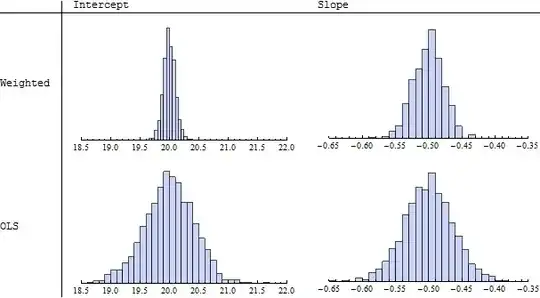
Because I specified an intercept of $20$ and slope of $-1/2$, we will want to use these values as references. Indeed, the histograms in the left column ("Intercept") display sets of estimated intercepts hovering around $20$ and the histograms in the right column ("Slope") display sets of slopes hovering around $-0.50 = -1/2$. This illustrates the theoretical fact that the estimates in either case are unbiased. However, looking more closely at the spreads of the histograms (read the numbers on the horizontal axes), we see that those in the upper row ("Weighted") have smaller widths of their counterparts in the lower row ("OLS," or "Ordinary Least Squares"). This is evidence that the weighted estimates tend, on the whole, to be better then the unweighted ones, because they tend to deviate less from the true parameter values.

When the underlying data truly conform to the hypothesized model--there is a linear relationship between the $x$'s and $y$'s, with errors in the $y$'s having known but differing standard deviations--then among all unbiased linear estimates of the slope and intercept, weighted least squares using reciprocal variances for the weights is best in the sense just illustrated.

Obtaining the estimation error of the slope

Now, to answer the question: we would like to assess the estimation error in the slope. This can be obtained from the fit object in many ways: consult the help page for details. Here is a nicely formatted table:

fit = LinearModelFit[y, t, t, Weights -> 1 / errors^2];
fit0 = LinearModelFit[y, t, t];
TableForm[{{fit[#], fit0[#]} & @ "ParameterConfidenceIntervalTable"}, 
  TableHeadings -> {{}, {"Weighted", "OLS"}}]

Tables

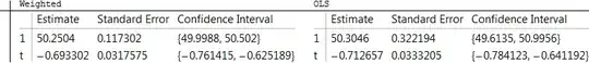
In this case, for this particular set of simulated data (as created previously), the weighted method reports a much smaller standard error for the intercept than the OLS method (because errors near $x=0$ are low according to the information in errors) but the weighted estimate of the slope has only a slightly smaller standard error than the OLS estimate of the slope.


Comments

Errors in both $x$ and $y$ can be handled, using--for instance--methods of maximum likelihood. However, this involves considerably more mathematical, statistical, and computational machinery and requires a careful assessment of the nature of those errors (such as whether the $x$ errors and $y$ errors are independent). One general result in the statistical literature is that when the $x$ errors are typically smaller than the $y$ errors, yet independent of them, it is usually safe to ignore the $x$ errors. For more about all this, good search terms include "errors-in-variables regression," "Deming regression," and even "principal components analysis (PCA)".

whuber
  • 20,544
  • 2
  • 59
  • 111
  • I posted a solution to the problem of errors in both $x$ and $y$ at http://stats.stackexchange.com/a/201915/919 . Although it is illustrated with R code, it is readily implemented in Mathematica. I believe it may be the same as the algorithm posted in this thread by J.M., but with some modifications to make it more robust and broadly applicable. In particular, (1) it provides a good starting value for the parameters (by finding an Ordinary Least Squares solution) and (2) it uses the angle of the fitted line rather than its slope as one of the parameters. – whuber Mar 16 '16 at 14:15
  • 1
    Actually, I had computed the line's slope in my answer by dividing a sine by a cosine (which was what FindArgMin[] was looking for in my routine), so it should not be too hard to modify my routine to return an angle instead if needed via two-argument arctangent. – J. M.'s missing motivation Jun 17 '16 at 15:11
  • using weights for this purpose is very bad idea. Say that all data points have the same uncertainty SE = 1. Then say that all data points have SE = 2. In both cases, weights are the same, so weighting will make no difference. But the uncertainty in the second example is twice as large, and this is apparently not taken into account. – Tomas Sep 25 '16 at 08:41
  • 1
    @Tomas The weighting does make a difference in standard errors, confidence intervals, and prediction intervals. I see little support for your conclusion that weighting is a "very bad idea." That conclusion must be based on some unstated assumptions, for otherwise it flies in the face of a well-established theory, which you can find in any textbook on regression. – whuber Sep 25 '16 at 19:26
  • @whuber I mean weighting for the purpose of incorporating uncertainty, not weighting in general. Rather than a well-established theory it seems like unfortunately common but very sloppy and desperate practice to somehow incorporate SEs. Why 1/SE and not 1/SE^2? Noone knows, it's just something to keep referees silent. I gave you an example in my previous comment why it is a complete nonsense. How do you respond to that? – Tomas Sep 26 '16 at 19:29
  • @Tomas It is not the case that this is "sloppy," "desperate," or that "noone knows." Please consult any regression textbook for an account of the theory and the assumptions that must be met. – whuber Sep 26 '16 at 19:30
  • @whuber 1) could you please provide a concrete reference that would justify the method? Not just use it, I know plenty of such studies. Statistically justify the method. Haven't found it in the textbooks I came accross :-) 2) so, the example I stated in my first comment here still goes without an answer? There should be answer to that, if the method is valid. – Tomas Sep 26 '16 at 19:35
  • 1
    @Tomas Montgomery, Peck, and Vining, Introduction to Linear Regression Analysis. Fifth Edition (Wiley), 2012. Section 5.5. – whuber Sep 26 '16 at 19:50
  • @whuber thanks, unfortunatelly I don't have access to this one. Do you have any arguments for the example I presented? – Tomas Sep 27 '16 at 12:05
13

I made this implementation of York's classical (and easy to understand) method following this paper by Cameron Reed.

f[x_List, y_List, wxi_List, wyi_List] :=
  Module[{n = Length@x, wi, ui, vi, wmean, d, g, a, b, set, least},

   wi[i_, m_]        := wxi[[i]] wyi[[i]]/(m ^2 wyi[[i]] + wxi[[i]]);
   ui[i_, m_]        := x[[i]] - wmean[x, m];
   vi[i_, m_]        := y[[i]] - wmean[y, m];
   wmean[q_List, m_] :=  Sum[wi[i, m] q[[i]], {i, n}]/Sum[wi[i, m], {i, n}];
   d[m_]             :=  Sum[wi[i, m]^2 ui[i, m]^2/wxi[[i]], {i, n}];
   g[m_]             :=- Sum[wi[i, m]   ui[i, m] vi[i, m], {i, n}]/d[m];
   a[m_]             :=2 Sum[wi[i, m]^2 ui[i, m] vi[i, m]/wxi[[i]], {i, n}]/(3 d[m]);
   b[m_]             := (Sum[wi[i, m]^2 vi[i, m]^2/wxi[[i]], {i, n}] - 
                         Sum[wi[i, m] ui[i, m]^2, {i, n}])/(3 d[m]);

   set = {ToRules@ Reduce[m^3 - 3 a[m] m m + 3 b[m] m - g[m] == 0 && 
                          c == wmean[y, m] - m wmean[x, m], {m, c}, 
                          Backsubstitution -> True]};

  least = Sum[wxi[[i]] (x[[i]] - (y[[i]] - c)/m)^2 + 
              wyi[[i]] (y[[i]] - (m x[[i]] + c))^2, {i, Length@x}] /. 
                set[[Flatten@Position[m /. set, _Real]]];

  set[[Flatten@Position[m /. set, _Real]]][[Position[least, Min@least][[1]]]]];

Usage

f[Range[10], 3 Range[10] + RandomReal[.2], Array[# &, 10], Array[# &, 10]]
(*
 -> {{m -> 3., c -> 0.110805}}
*)
Dr. belisarius
  • 115,881
  • 13
  • 203
  • 453
  • This solution doesn't seem to work for all data. Changing the x error list to "{1, 2, 3, 4, 5, 6, 7, 8, 9, 2}" makes f return an error and a long, weird solution. Pastebin: http://pastebin.com/dMzTjweu – George S Oct 16 '12 at 03:40
  • @GeorgeS I forgot to filter out imaginary results. Fixed now – Dr. belisarius Oct 16 '12 at 03:58
  • I still receive the same error. The data I am using: f[{2.04, 3.06, 4.08, 5.1, 6.12, 7.14, 8.16}, {1.9975, 3.216, 4.0939, 4.9878, 6.4685, 7.2003, 8.2944}, {0.02, 0.03, 0.04, 0.05, 0.06, 0.07, 0.08}, {0.1696, 0.1793, 0.1821, 0.2568, 0.4197, 0.1342, 0.2304}] – George S Oct 16 '12 at 05:11
  • I'm probably missing something, but shouldn't it be possible to obtain the error estimates for m and c? – Ajasja Oct 16 '12 at 09:43
  • @Ajasja, yes, the formulae are in York's paper... – J. M.'s missing motivation Oct 16 '12 at 10:00
  • @J.M. Yes, they are a sum away in the paper I cited at the beginning. Being this a HW question I think some work should be left to the OP – Dr. belisarius Oct 16 '12 at 10:28
  • @belisarius Aaa, sorry, I missed the homework part. – Ajasja Oct 16 '12 at 10:42
  • @GeorgeS Fixed with BackSubstitution->True . The Reduce[]command was giving c as a function of m. – Dr. belisarius Oct 16 '12 at 11:32
9

I'd take the simplest approach : solve the usual least-squares problem to determine the coefficients of the line; they will depend on the input data $(x_i, y_i)$. If the input data has an uncertainty $(dx_i, dy_i)$ then we can propagate it to the solution for the coefficients. We can do all this symbolically and substitute numerical values at the very end.

nPoints = 10;
data = Table[{Subscript[x, i], Subscript[y, i]}, {i, nPoints}];
errors = Table[{Subscript[dx, i], Subscript[dy, i]}, {i, nPoints}];

model[a_, b_, x_] = a x + b;

(* The least-squares functional; can be different, i.e. actual distance to the line *)
objFun[a_, b_, data_] := Total[(#[[2]] - model[a, b, #[[1]]])^2 & /@ data]

(* The usual solution *)
solab = First@Solve[{D[objFun[a, b, data], a] == 0, 
                     D[objFun[a, b, data], b] == 0}, {a, b}] ;

(* The squared deltas relative to the input data *)
deltaa = Flatten@{D[a /. solab, #]^2 & /@ data[[All, 1]] , 
                  D[a /. solab, #]^2 & /@ data[[All, 2]]};
deltab = Flatten@{D[b /. solab, #]^2 & /@ data[[All, 1]] , 
                  D[b /. solab, #]^2 & /@ data[[All, 2]]};

(* The error is the sum of delta times uncertainty, assuming independence *)
errora = Sqrt[Dot[deltaa, Flatten[errors]^2]];
errorb = Sqrt[Dot[deltab, Flatten[errors]^2]];

Now we can use our actual numeric data and substitute them everywhere in the above :

ndata = Sort@RandomReal[{-2, 2}, {nPoints, 2}];
nerrors = RandomReal[{0, 0.2}, {nPoints, 2}];

nmodel[x_] = model[a, b, x] /. (solab /. Thread[Rule[Flatten[data] , Flatten[ndata]]])
nsolab = solab /. Thread[Rule[Flatten[data] , Flatten[ndata]]]
nerrorab = {errora, errorb} //. Join[Thread[Rule[Flatten[data] , Flatten[ndata]]], 
                                      Thread[Rule[Flatten[errors] , Flatten[nerrors]]]]

(* -0.481409 + 0.125842 x
   {a -> 0.125842, b -> -0.481409}
   {0.0463579, 0.0385911} *)

Finally we can plot the data together with the best fit and the model corresponding to changing the parameters by $\pm$ 1 standard deviation.

Needs["ErrorBarPlots`"]

Show[Plot[{model[(a /. nsolab) - nerrorab[[1]], (b /. nsolab) - nerrorab[[2]], x], 
           model[(a /. nsolab) - nerrorab[[1]], (b /. nsolab) + nerrorab[[2]],x],    
           model[(a /. nsolab) + nerrorab[[1]], (b /. nsolab) - nerrorab[[2]], x], 
           model[(a /. nsolab) + nerrorab[[1]], (b /. nsolab) + nerrorab[[2]],x],  
           nmodel[x]}, {x, -2, 2}, PlotStyle -> {Dashed, Dashed, Dotted, Dotted, Red}, PlotRange -> All], 
     ErrorListPlot[Transpose[{ndata, ErrorBar @@@ nerrors}]]]   

enter image description here

b.gates.you.know.what
  • 20,103
  • 2
  • 43
  • 84
  • 1
    This seems to be conceptually contradictory: the OLS solution assumes one error structure, then you propagate different errors. Why should that work at all? – whuber Oct 15 '12 at 15:46
  • @b.gatessucks I seem to be unable to run this example properly. Running it when the random data your code uses, or pasting in my data returns a lot of errors. After a long delay, a graph with all the points but no lines of best fit appears. Pastebin: http://pastebin.com/xG9R79UN – George S Oct 16 '12 at 01:51
  • @GeorgeS You need a ; after the definition of ndata or use different cells for ndata and nerrors. Also you need to adjust the plot range. – b.gates.you.know.what Oct 16 '12 at 08:08
1

Here is a simplistic approach, but perhaps it is one step on from examining just the end points. It makes the assumption that nothing is known about the distribution of x, y errors other than they are uniform, if they are not uniformly distributed the problem becomes significantly more complex.

Data

Some experimental data:

data = {Range@(size + 1),Sin@Range[0, (2 \[Pi])/3, (2 \[Pi])/(3 size)]}//Transpose;

Errors

A vector of {xErr,yErr} pairs which represent the estimated, or measured, magnitude of mean error for x and y measurements at each value of x:

errorDeltas = ConstantArray[{.1, 0.2}, Length@data];

Here the values of mean x and y errors have been chosen to be constant, but from experimental data they might well be variable.

Uniform

The simplicity derived from the uniform assumption is that the errors are symmetric, so the aggregate effect, of rotation or translation, on the linear fit cancel out. This allows for a simple addition of the mean error vector to the data to represent a least squares solution.

model = LinearModelFit[data + errorDeltas, x, x]

Plotted

Show[ListLinePlot[data, PlotStyle -> Dashed], 
 Plot[model[x], {x, 1, Length@data}], PlotRange -> All]

Mathematica graphics

image_doctor
  • 10,234
  • 23
  • 40
  • I don't understand how one the method used; why would adding error to the data help? In addition, the solution doesn't estimate an error on the slope of the line, as is necessary. – George S Oct 16 '12 at 02:05
  • @GeorgeS This is a refinement of the example method you gave in your question using end points where the errors were added to the data. If the statistical distribution of the individual errors is uniform, or symmetric, then most likely ( maximum likelihood ) error value is the mean value of the errors. Thus, the most likely linear regression is the data plus the most likely error. The difference between this linear regression and the linear regression of the data on it's own, gives the error at any point on the regression. I hope that explanation wasn't too confusing :) – image_doctor Oct 16 '12 at 08:02
0

This is a slightly modified version(to amend its somehow strange error/uncertainty estimation behavior (which might be the result of some bug?)) of the answer of @J.M. I didn't found some place/website to store and share the codes (based on Krystek/Anton ) below so I post here instead (this is more likely a discussion then an answer):

ortlinfitmk2[data_?MatrixQ, errs_?MatrixQ] := 
Module[{n = Length[data], c, ct, dk, dm, k, m, p, s, st, ul, vl, w, 
wt, xm, ym, covmm, covkk, covmk, covkm},(*yes,
I know I could have used FindFit[] for this...*){ct, st, k} = 
Flatten[MapAt[Normalize[{1, #}] &, 
  NArgMin[Norm[
    Function[{x, y}, y - \[FormalM] x - \[FormalK]] @@@ 
     data], {\[FormalM], \[FormalK]}], 1]];
(*find orthogonal regression coefficients*){c, s, p} = 
 FindArgMin[{Total[(data.{-\[FormalS], \[FormalC]} - \
\[FormalP])^2/((errs^2).{\[FormalS]^2, \[FormalC]^2})], \[FormalC]^2 \
+ \[FormalS]^2 == 1}, {{\[FormalC], ct}, {\[FormalS], 
   st}, {\[FormalP], k/ct}}];
(*slope and intercept*)
{m, k} = {s, p}/c;
wt = 1/errs^2; w = (Times @@@ wt)/(wt.{1, m^2});
{xm, ym} = w.data/Total[w];
ul = data[[All, 1]] - xm; vl = data[[All, 2]] - ym;
(*uncertainties in slope and intercept*)
dm = w.(m ul - vl)^2/w.ul^2/(n - 2);
dk = dm (w.data[[All, 1]]^2/Total[w]);

covmm = 
Total@MapThread[
  1/(m^2 #1[[1]]^2 + #1[[
       2]]^2)^3 2 ((m^2 #1[[1]]^2 + #1[[2]]^2)^2 #2[[1]]^2 - 
      4 m #1[[1]]^2 (m^2 #1[[1]]^2 + #1[[2]]^2) #2[[
        1]] (k + m #2[[1]] - #2[[2]]) + 
      4 m^2 #1[[1]]^4 (k + m #2[[1]] - #2[[2]])^2 - #1[[
        1]]^2 (m^2 #1[[1]]^2 + #1[[2]]^2) (k + 
         m #2[[1]] - #2[[2]])^2) &, {errs, data}];
 covkm = 
 Total@MapThread[(-4 k m #1[[1]]^2 - 2 m^2 #1[[1]]^2 #2[[1]] + 
    2 #1[[2]]^2 #2[[1]] + 
    4 m #1[[1]]^2 #2[[2]])/(m^2 #1[[1]]^2 + #1[[2]]^2)^2 &, {errs,
    data}];
 covmk = 
 Total@MapThread[(-4 k m #1[[1]]^2 - 2 m^2 #1[[1]]^2 #2[[1]] + 
    2 #1[[2]]^2 #2[[1]] + 
    4 m #1[[1]]^2 #2[[2]])/(m^2 #1[[1]]^2 + #1[[2]]^2)^2 &, {errs,
    data}];
 covkk = 
 Total@MapThread[2/(m^2 #1[[1]]^2 + #1[[2]]^2) &, {errs, data}];
 {Function[\[FormalX], Evaluate[{m, k}.{\[FormalX], 1}]], 
 Sqrt[{dm, dk}], 
 Sqrt@Diagonal[2*Inverse@{{covmm, covkm}, {covmk, covkk}}]}] /; 
 Dimensions[data] === Dimensions[errs]

(I really don't understand the code where dm and dk are calculated in ortlinfit @J.M. (due to my poor mathematica experience and math base))

then with

data = {{0, 5.9}, {0.9, 5.4}, {1.8, 4.4}, {2.6, 4.6}, {3.3, 
3.5}, {4.4, 3.7}, {5.2, 2.8}, {6.1, 2.8}, {6.5, 2.4}, {7.4, 1.5}};

errs = {{1000., 1.}, {1000., 1.8}, {500., 4.}, {800., 8.}, {200., 
 20.}, {80., 20.}, {60., 70.}, {20., 70.}, {1.8, 100.}, {1, 
 500.}} // Sqrt[1/#] &;

the covkms in the code above are the result of something like (Hessian matrix (18) in the Krystek/Anton)

x2 = (yk - xk m - k)^2/(uxk^2 m^2 + uyk^2)
Outer[D[x2, #1, #2] &, {m, k}, {m, k}] // FullSimplify // MatrixForm

I replaced uxks to #s manually.

we have

fitanderr = ortlinfitmk2[data, #*errs] & /@ (2^Range@8)

{{Function[\[FormalX]$, 5.47991 - 0.480533 \[FormalX]$], {0.0710065, 
0.361871}, {0.115143, 0.584743}},...,
{Function[\[FormalX]$, 5.47989 - 0.480528 \[FormalX]$], {0.0710063, 
0.361871}, {14.7381, 74.8463}}}

then

ListLogPlot[{Transpose[{2^Range@8, fitanderr[[All, 2, 1]]}], 
Transpose[{2^Range@8, fitanderr[[All, 3, 1]]}]}, Joined -> True, 
AxesLabel -> {"#*err", "dm"}, LabelStyle -> 12, 
PlotLegends -> 
Placed[{"dm ortlin", "dm ortlinmk"}, Scaled[{.5, .4}]]]

gives

enter image description here

obviously the dm of ortlinfitmk2 is more reasonable.

Harry
  • 2,715
  • 14
  • 27