2

I need to find the roots of a nonlinear function, namely:

F[z_] = 2 E^(2 I b z)
z ((-1 + E^(2 I a Sqrt[z^2 - Subscript[V, 0]])) z + (1 + E^(
    2 I a Sqrt[z^2 - Subscript[V, 0]])) Sqrt[
  z^2 - Subscript[V, 0]]) + (E^(2 I a z) - E^(2 I b z)) (-1 + E^(
 2 I a Sqrt[z^2 - Subscript[V, 0]])) Subscript[V, 0]   

where:

$\omega$ is complex valued and $a,V_{0}, b$ are real parameters.

I've been trying to solve numerically this problem by defining a new function

G[x_, y_] := Module[{Z}, Z = x + I*y; Abs[N[1/F[Z]]]]

making a contour plot of this and then approximating the roots by FindRoot

ContourPlot[G[x, y], {x, -10, 10}, {y, -4, 4},PlotLegends -> Automatic, 
FrameLabel -> {"x", "y"}, Mesh -> False, MaxRecursion -> 5]

but it's not giving me the better graphical quality that I need. Is there any better way to evaluate these complex roots?
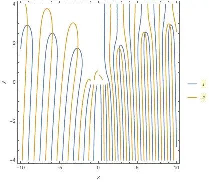
J. M.'s missing motivation
  • 124,525
  • 11
  • 401
  • 574

1 Answers1

1

Not sure why G deals with the reciprocal of F, but taking F as the function whose roots are desired, as indicated in the first sentence, I get this:

Block[{b = 1, Subscript, a = 1},
 Subscript[V, 0] = 1;
 NSolve[F[z] == 0 && -10 < Re[z] < 10 && -4 < Im@z < 4, z]
 ]
(*
  {{z -> -9.16236 + 2.93903 I}, {z -> -5.94891 + 2.52432 I},
   {z -> -2.66633 + 1.75482 I}, {z -> 2.66633 + 1.75482 I},
   {z -> 5.94891 + 2.52432 I}, {z -> 9.16236 + 2.93903 I}}
*)

Plot:

Block[{b = 1, Subscript, a = 1},
 Subscript[V, 0] = 1;
 ContourPlot[
  Evaluate@Thread[ReIm[F[x + I y]] == 0], {x, -10, 10}, {y, -4, 4}, 
  PlotLegends -> Automatic, FrameLabel -> Automatic, MaxRecursion -> 3]
 ]

Mathematica graphics

Michael E2
  • 235,386
  • 17
  • 334
  • 747
  • Thank you, it works nicely! Just one more question., do you have any idea about how could I make a graph of this this function? @MichaelE2 – Herr Schrödinger Dec 14 '16 at 00:43
  • 1
    @WaynerKlën See my update. See if that is what you want. – Michael E2 Dec 14 '16 at 01:57
  • What do the lines represent? – Herr Schrödinger Dec 14 '16 at 02:11
  • 1
    @WaynerKlën Re@F[z] == 0 and Im[F[z]] == 0. Look up ReIm in the docs (unless you have an old version of Mma). Perhaps you'd like a plot of several contours? If so, which ones? The traditional ones are the real part, imaginary part, absolute value (modulus), and argument. Just apply the appropriate function to F[x + y I] and omit the equality == 0 – Michael E2 Dec 14 '16 at 02:44
  • What does each axis mean? Would it be the x axis real part of $\omega$ and the y axis the imaginary part of $\omega$? – Herr Schrödinger Dec 22 '16 at 16:04
  • 1
    They are the axes of the argument x + I y in F[x + I y]], which would be real and imaginary parts of z = x + I y. The OP does not say how $\omega$ is related to the code, but if it is the same as z, then the answer to your 2nd question is yes. – Michael E2 Dec 22 '16 at 16:27
  • Yeah @MichaelE2, $z=\omega$, but if the both axes are related to the argunments of $z$ the graph of this function shouldn't be a 3-dimensional obejct?Just to clarify my mind. – Herr Schrödinger Dec 22 '16 at 16:33
  • 1
    @WaynerKlën, most generally the equation w = F[z], with z and w complex, defines a surface in ${\bf R}^4 = {\bf C}^2$, which cannot be plotted (easily) on a screen. The plot in my answer plots two curves, Re[F[x + I y]] == 0 and Im[F[x + I y]] == 0; the intersections are where F == 0. Perhaps you're looking for something like Plot3D[Abs[F[x + I y]], {x, -10, 10}, {y, -4, 4}]? There are various ways for trying to visualize complex functions. (P.S. I just realized I forgot to convert my plot code back to Subscript[V, 0].) – Michael E2 Dec 22 '16 at 16:54
  • Your Answer was very good, but I need to justify why this plot represents something acceptable. I just didn't understand one thing: It looks like to me that you take $F(z)==constant$ and made the plot, this way I can figure that plot, is this it? – Herr Schrödinger Dec 22 '16 at 17:03
  • 1
    @WaynerKlën Yes, but for a nonzero $constant$, I would write it as $F(z) - constant == 0$ in the code, and use Evaluate@Thread[ReIm[F[x + I y] - constant] == 0] for the plot. (You don't need to do that for NSolve.) – Michael E2 Dec 22 '16 at 17:08