3

I have to solve a transcendental equation for a parameter, say $\beta$. Now, the $\beta$ has a range from $ik$ to $k$ where $i$ is the usual imaginary root $\sqrt{-1}$ and $k$ is a real number. Problem is, the transcendental equation has multiple solutions, and so I cannot guess what will be the proper choice for the initial value of $\beta$ in FindRoot. I could do it if $\beta$ ranges from $p$ to $q$ where $p$ and $q$ are reals by plotting the transcendental equation's lhs and rhs. However, I don't know how to plot complex ranges. Is there any way to guess the initial values?


Code I used:

e1 = 1; e2 = -1; e0 = 8.854*^-12; mu0 = 1.257*^-6; c = 3.0*^8; w = 2*Pi*2*^14;
k = w/c; a = 600*^-9; k1 = w*Sqrt[e1]/c; k2 = w*Sqrt[e2]/c; b = p + q I;
u = Sqrt[k1^2 - b^2]; ww = Sqrt[b^2 - k2^2]; v = 1;

t1 = (BesselJ[v - 1, u a] - BesselJ[v + 1, u a])/(2*u*BesselJ[v, u a]);
t2 = -(BesselK[v - 1, ww a] + BesselK[v + 1, ww a])/(2*ww* BesselK[v, ww a]);

x = (e1 t1 + e2 t2) (t1 + t2); y = ((b*v)/(k*a))*(1/u^2 + 1/ww^2);

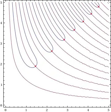
ClickPane[ ContourPlot[{Re[x - y^2], Im[x - y^2]}, {p, 0, k}, {q, 0, k}],
(xycord = #) & ] Dynamic[xycord]
J. M.'s missing motivation
  • 124,525
  • 11
  • 401
  • 574
4208
  • 33
  • 4
  • Here's a way to plot complex numbers, so you may be able to get a feel for good values: http://mathematica.stackexchange.com/questions/16252/plotting-complex-numbers – bill s Apr 10 '13 at 19:47
  • can you give a simple example? – Spawn1701D Apr 10 '13 at 20:07
  • say the equation is x=y where x and y contains bessel functions and its derivatives. I have to solve it for beta. If beta ranges from p to q where p and q are real numbers. I could write Plot[{x,y},{beta,p,q}] Then from the plot i get a feel for good values. But ik to k (where i is the usual imaginary root sqrt(-1) and k is a real number) is the allowed range for beta* and i cannot write Plot[{x,y},{beta,i*k,k}] it surely gives me error! By using FindRoot[x==y,{beta,_initial value_}] I get solution though but changing initial value just a little beta changes completely. – 4208 Apr 10 '13 at 22:20

1 Answers1

6

One method I use is to separately plot the zero contours of the real and imaginary parts of the equation whose complex roots are being sought.

As a particular example, say I want the complex roots $z=x+iy$ of the error function,

$$\mathrm{erf}(z)=0$$

in the first quadrant, $0<x,y<5$.

I do something like this:

plt = ContourPlot[{Re[Erf[x + I y]] == 0, Im[Erf[x + I y]] == 0}, {x, 0, 5}, {y, 0, 5}]

contours of real and imaginary parts

One option is manual: right-click on the image, click "Get Coordinates", pick out and click on a crossing, and then press Ctrl+C to copy the coordinates. For instance, if I want the root of least magnitude, my attempt at performing that procedure yields the point {1.453, 1.887}, which can then be fed to FindRoot[]:

FindRoot[Erf[z] == 0, {z, 1.453 + 1.887 I}]
   {z -> 1.450616163243677 + 1.8809430001533158*I}

A better approach to finding these roots is to use a utility function called FindAllCrossings2D[] due to Stan Wagon. Here's how to use it:

sols = FindAllCrossings2D[{Re[Erf[x + I y]], Im[Erf[x + I y]]}, {x, 0, 5}, {y, 0, 5}]
   {{1.4506161632436756, 1.8809430001533154}, {2.2446592738032476, 2.61657514068944},
    {2.839741046908047, 3.175628099643187}, {3.3354607354411554, 3.646174376387361},
    {3.7690055670142044, 4.060697233933308}, {4.158998399781451, 4.435571444236523},
    {4.516319399583921, 4.78044764414843}}

Conversion to the corresponding complex roots is easy, of course:

#1 + I #2 & @@@ sols

You can graphically verify the roots, too:

Show[plt, Epilog -> {AbsolutePointSize[4], Red, Point[sols]}]

contours and roots

J. M.'s missing motivation
  • 124,525
  • 11
  • 401
  • 574