A hint for an exact solution of a system of differential equations

Question

I am looking for a curve in two-dimensional space, so $c(t)=(x(t),y(t))$, that satisfies a system of differential equations which could not be solved with Mathematica $$ x''(t) = (k - c \; y(t))\; y'(t) \\ y''(t) = -(k - c \; y(t))\; x'(t) $$ The differential equations enforce that $c''(t)$ is perpendicular to $c'(t)$, so it is clear that $c'(t)$ always has constant length and it may be assumed this length is $1$.

The constants $k$ and $c$ are both positive. I am interested especially in the case where $k$ is about $1/4$ and $c$ is about $4/1000$, but I think it can be solved with arbitrary positive $k$ and $c$.

The differential equations can be solved quite good numerically. And I know from numerical computations that a prolate cycloid has nearly the same orbit (path) as the seeked curve. Unfortunately the solution is only nearly a prolate cycloid. One deficiency of a prolate cycloid is that it doesn't have constant velocity $|c'(t)|$.

I would be very glad, if someone could give me a hint to solve these equations.

Answer 1

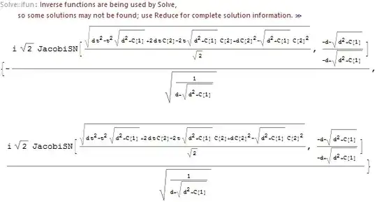
Symbolic solution

Even though Mathematica cannot solve straightforwardly the original system we can get the symbolic solutions with a little bit smarter approach. Let's observe that we can get rid of x'[t] and x''[t] from the system by changing variables y -> z[t] == k - c y[t], thus z'[t] == -c y'[t] and z''[t] == -c y''[t] therefore x''[t] == (k - c y[t]) y'[t] implies that x''[t] == -1/c z[t] z'[t], integrating it we get c x'[t] + 1/2 z[t]^2 + d == 0, where d is a constant of integration. Inserting this into the second equation yields

    z''[t] + 1/2 z[t]^3 + d z[t] == 0

This equation can be solved in terms of Jacobi elliptic functions:

sols = z[t] /. DSolve[{z''[t] + 1/2 z[t]^3 + d z[t] == 0}, {z[t]}, {t}]

Recalling that z[t] == k - c y[t] we can easily figure out periodic-like behaviour of y[t] found in numerical calculations. In order to get x[t] we need inserting y[t] into the original system, then integrating with respect to t. It seems that we should work with appropriate initial conditions y[0] and y'[0] and choose adequate branches of solutions. Then various special cases could clarify the overall behaviour of the system, let's consider a special case.

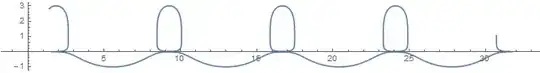
 sd041 = FullSimplify[sols /. {d -> 0, C[1] -> 4, C[2] -> 1}, t > 0]

{-2 JacobiSN[1 + t, -1], 2 JacobiSN[1 + t, -1]}

Taking the second equation of the original system we can get x'[t] (assuming c == 1 and k == 1):

FullSimplify[ D[ sd041[[1]], {t, 2}]/(1 - sd041[[1]]), t > 0]

(4 JacobiSN[1 + t, -1]^3)/(1 + 2 JacobiSN[1 + t, -1])

and x[t] is (putting the constant of integration equal to zero):

xx = Integrate[(4 JacobiSN[1 + t, -1]^3)/(1 + 2 JacobiSN[1 + t, -1]), t]

We plot only the real part of xx as x[t], (this is because of another issue, see e.g. Why does Integrate declare a convergent integral divergent? )

Plot[{ Re @ xx, 1 - sd041[[1]]}, {t, 0, 20}]

and the solution in the phase space is

ParametricPlot[{ Re @ xx, 1 - sd041[[1]]}, {t, 0, 20}]

At this point it is plausible to exploit numerical capabilities of the system

Numerical solution

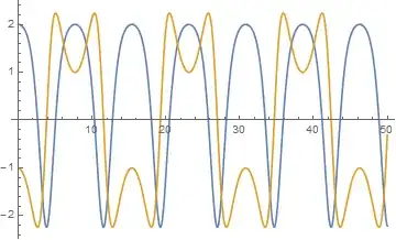
We can exploit NDSolve and including arbitrary initial conditions, we can compare various cases:

With[{c = 1/4, k = 4/1000}, 
     ds = NDSolve[{x''[t] == (k - c y[t]) y'[t], 
                   y''[t] == -(k - c y[t]) x'[t], 
                   x[0] == 1, y[0] == 0, x'[0] == 2, y'[0] == -1},
                   {x[t], y[t]}, {t, 0, 150}]];
{X[t_], Y[t_]} = {x[t], y[t]} /. First @ ds;

Now we plot the solution in the range 0 < t < 50:

Plot[{X[t], Y[t]}, {t, 0, 50}]

as well as its derivative

Plot[{X'[t], Y'[t]}, {t, 0, 50}]

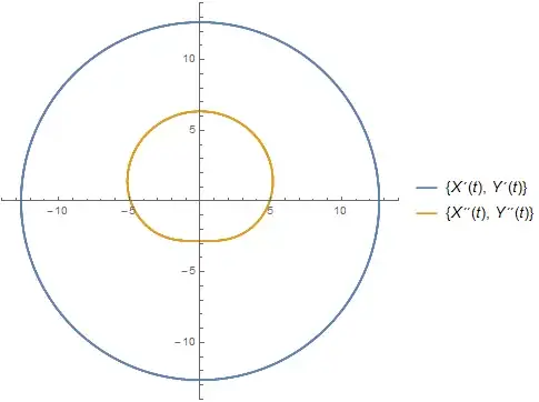
Another interesting feature can be observed with the parametric plot of the solution:

ParametricPlot[{X[t], Y[t]}, {t, 0, 60}]

and it is expected to compare the first and the second derivatives of the solution, we can do it with the animated parametric plot:

tab = 
 Table[ ParametricPlot[{{X'[t], Y'[t]}, {X''[t], Y''[t]}}, {t, 0, v}, 
          PlotLegends -> Placed[Style[Row[{"t = ", NumberForm[N@v, {3, 1}]}],
                                        Bold, 20], {Left, Top}], 
          PlotRange -> {{-3.5, 3.5}, {-3.5, 3.5}}], {v, 1, 16, 1/6}];

ListAnimate[ tab, Paneled -> False]

Edit

The OP expected solutions with reversed values (c == 4/1000, k == 1/4) Then the system behaves in a different way:

With[{c = 4/1000, k = 1/4}, 
     ds = NDSolve[{x''[t] == (k - c y[t]) y'[t], 
                   y''[t] == -(k - c y[t]) x'[t], 
                   x[0] == -16, y[0] == 4, 
                   x'[0] == 12, y'[0] == -4}, {x[t], y[t]}, {t, 0, 130}]];
 {X[t_], Y[t_]} = {x[t], y[t]} /. First@ds;

Now the phase space solution is more similar to cycloid-like

ParametricPlot[{X[t], Y[t]}, {t, 0, 100}]

 ParametricPlot[{{X'[t], Y'[t]}, 
                {X''[t], Y''[t]}}, {t, 0, 100}, 
                PlotLegends -> "Expressions"]

Playing with different initial conditions we can get various patterns of the behaviour, more or less similar to the previous case with {c = 1/4, k = 4/1000}. Nonetheless from programming point of view the task of examining the system is the same.

Answer 2

Analytical solution with Maple

Maple is able to produce an analytical solution with out the use of the initial conditions,

restart;
Eq1:= diff(x(t),t$2)=(k-c*y(t))*diff(y(t),t$1):
Eq2:= diff(y(t),t$2)=-(k-c*y(t))*diff(x(t),t$1):
dsolve({Eq1,Eq2});

But, if when we specify only two initial conditions ,

sol1:=dsolve({Eq1,Eq2,x(0)=a1,y(0)=b1});

odetest(sol1,{Eq1,Eq2,x(0)=a1,y(0)=b1})

{0}

If we can take another combination of the conditions,

sol2:=dsolve({Eq1,Eq2,x(0)=a1,D(x)(0)=c1});

odetest(sol2,{Eq1,Eq2,x(0)=a1,D(x)(0)=c1})

{0}

With these combinations y(0)=b1,D(y)(0)=d1 and D(x)(0)=c1,D(y)(0)=d1 maple produces no output.

Mathematica's DSolve is unable to solve the system in question analytically.

Numerical solution with Mathematica

C1 = 4/1000; K1 = 1/4;

sol1[x0_?NumericQ] := 
  First@NDSolve[{x''[t] == y'[t]*(K1 - C1*y[t]), 
     y''[t] == -x'[t]*(K1 - C1*y[t]), x[0] == x0, x'[0] == x0, 
     y[0] == x0, y'[0] == x0}, {x, y}, {t, -10, 10}];

ParametricPlot[
 Evaluate[{x[t], y[t]} /. sol1[#] & /@ Range[-10, 10, 1]], {t, -10, 
  10}, Frame -> True, PlotRange -> All]

Answer 3

First I appreciate the revision of my initial question done by Artes. It is much clearer now. Further I thank all who gave me hints for analytical solutions. In the end I had to accept that there is no really simple solution --- as I posted my question, I had the hope there might be a solution which I just can see even it is not to intricate.

After all I had to go back to a numerical solution and I'll describe my proceeding as it is strait forward and can even be carried out on Excel:

I start with a initial condition c(0) and c'(0) [c'(0) with length 1] and the differential equation gives me c''(0) as

x′′(0)=(k−cy(0))y′(0)
y′′(0)=−(k−cy(0))x′(0).

Now for a small t I get

x'(t)=x'(0)+t*x''(0)
y'(t)=y'(0)+t*y''(0).

I normalize c'(t) to length 1 and take the mean value mv(t) = (c'(0)+c'(t))/2, which I normalize likewise. Then I count

x(t)=x(0)+t*mvx(t)
y(t)=y(0)+t*mvy(t),

where mvx is the x-part of mv an mvy is the y-part of mv. Then I do the same procedure with starting point c(t) and c'(t) to get values for 2*t and so on ...

In this way I get c(n*t) for n=0, 1, 2, 3, ... If t is small enough this will be a fine approximation to the real solution.