How to generate a RandomVariate of a custom distribution?

Question

I'm trying to generate a pseudorandom variate out of a custom distribution. Suppose I want define a custom distribution, and for the sake of simplicity I define a Poisson distribution (the distribution I want is a derived mixture of two Poisson distributions):

custom[a_] := ProbabilityDistribution[(a^k Exp[-a])/k!, {k, 0, ∞, 1}];

When I now try to generate a RandomVariate[] of that distribution,

RandomVariate[custom[2], 10]

I obtain the following error:

RandomVariate::noimp: Sampling from ProbabilityDistribution[2^x/(E^2 x!),{x,0,∞,1}] is not implemented.

For the record, when the distribution is defined as a continuous distribution:

custom[a_] := ProbabilityDistribution[(a^k Exp[-a])/k!, {k, 0, ∞}];

there is no problem with the use of RandomVariate.

I'd appreciate some insight into this problem, thanks!

Answer 1

The short answer is: I don't think it is built to always work for general distributions (though see Sjoerd C. de Vries's answer and continuous example below).
You might also want to have a look at the nice tutorial how to Create Your Own Distribution with Oleksandr Pavlyk.

Lets see what are your options

Mixture

For mixture distributions, following J. M., we can define a mixture as:

DD[μ_, ν_, a_, b_] =
               MixtureDistribution[{a, b}, {PoissonDistribution[μ], PoissonDistribution[ν]}]

so that

RandomVariate[DD[4, 3, 1, 2], 16]

(* {5, 5, 6, 3, 5, 7, 9, 1, 3, 7, 5, 5, 3, 5, 2, 3} *)

Transformation

One can also use TransformedDistribution to define a new distribution from a known one, and draw from it:

RandomVariate[TransformedDistribution[x - 4,
  x \[Distributed] PoissonDistribution[10]] // Release, 15]

Draw via Cumulative Distrubution

For a set of distributions for which the cumulative distribution exists, within which your example falls (though it probably differs from what you really want to do), the inverse of the cumulative distribution can be used to define a draw:

 CDF[custom[a], x]

 (* Gamma[1 + Floor[x], a]/Gamma[1 + Floor[x]] *)

So for instance,

  g[x_] = CDF[custom[10], x];
  h = Table[{g[x], x}, {x, 0, 40}] // N // Interpolation[#, InterpolationOrder -> 0] &;

which allows us to define the inverse of the CDF:

  h /@ (RandomReal[{0, 1}, {12}])

  (*  {12., 15., 6., 17., 12., 8., 6., 9., 8., 13., 13., 12.} *)

  Show[h /@ (RandomReal[{0, 1}, {125000}]) // Histogram[#, Automatic, "Probability"] &, 
       Plot[PDF[custom[10], x - 1/2], {x, 0, 20}]]

Empirical Distribution

For a more general class of distribution, there is a twisted route within the current set of existing Mathematica functions: if you can draw samples which satisfy the distribution, then you can derive an EmpiricalDistribution (thanks J. M.) from your sample and then draw through it. It might be useful if it's costly to draw in the first place.

Continuous distribution where ProbabilityDistribution works with Random Variate

norm = Integrate[Exp[-x^2]/(c^2 + x^2), {x, -Infinity, Infinity},Assumptions -> c > 0]; 
DD[c_] = ProbabilityDistribution[1/norm Exp[-x^2]/(c^2 + x^2),
  {x, -Infinity,Infinity},Assumptions -> c > 0];

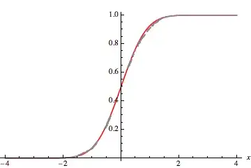
Let's check that the random variate sample is consistent

 data =RandomVariate[DD[4], 1500];

 DDE = EmpiricalDistribution[data];
 {Plot[CDF[DD[4], x] // Release, {x, -4, 4},PlotStyle -> Directive[Red]], 
  Plot[CDF[DDE, x], {x, -4, 4}]} // Show

Note that it can involve more than one parameter:

 norm = Integrate[Exp[-β x^2]/(c^2 + x^2),{x,-Infinity,Infinity},Assumptions->{c > 0, β>0}];
 DD[c_, β_] = ProbabilityDistribution[1/norm Exp[-β x^2]/(c^2 + x^2),
  {x, -Infinity, Infinity}, Assumptions -> (c > 0 && β > 0)];

 RandomVariate[DD[1, 1], 4]

 (* {0.149204,-0.644442,-0.632239,-0.266628} *)

Final Note

For 2D generalization see RandomVariate from 2-dimensional probability distribution

Answer 2

I have a hunch that the problem lies in the use of Infinity in combination with a finite step. So, it's not an issue of continuous vs discrete. Replace $\infty$ with a sufficiently large number (with the factorial involved 100 should be OK) and it works:

custom[a_] := ProbabilityDistribution[(a^k Exp[-a])/k!, {k, 0, 100, 1}];

RandomVariate[custom[2], 10]

{2, 2, 1, 4, 2, 2, 1, 4, 1, 1}

Let's test whether a set of 10 million random draws from the custom distribution are described by a Poisson distribution with the same parameter:

EstimatedDistribution[RandomVariate[custom[2], 10000000], PoissonDistribution[λ]]

PoissonDistribution[1.9999276]

EstimatedDistribution[RandomVariate[custom[8.5], 10000000], PoissonDistribution[λ]]

PoissonDistribution[8.5006323]

Answer 3

This is trivially easy with mathStatica for Mathematica, for ANY arbitrary discrete distribution. For the original poster's problem:

f = Exp[-a] a^x / x!;
domain[f] = {x, 0, Infinity} &&  {a > 0}  &&  {Discrete};

Here are 10 pseudo-random drawings:

RandomNumber[10, f /. a -> 2]
{2, 2, 1, 4, 3, 0, 1, 1, 1, 7}

And here are 100,000 more:

data = RandomNumber[100000, f /. a -> 2];

Next, compare a frequency plot of the empirical sample data we have just generated (the red dots) to the parent symbolic pmf (in blue):

FrequencyPlotDiscrete[data, f /. a -> 2]

Splendido. Just as easy for anything else :)

We have a chapter on these sorts of issues... see Chapter 3 of: Rose and Smith (Nov. 2011), Mathematical Statistics with Mathematica.