Visualization of numerical integration

Question

I have to do a project about numerical integration. My problem is visualizing my method.

My code:

Begin["private`"]
CMp[g_, y1_, y2_, m_] := 
  Module[{i = 0, summ = 0},
    While[i < m, summ = summ + g[y1 + i*(y2 - y1)/m]; i++];
    Return[N[summ*(y2 - y1)/m]]]

My teacher told me that I had to draw a integrand plot with m rectangles on it. I have no idea how can I do this. Any help?

Make rectangles of width equal to your iteration step and height equal to your function and display them side-by-side. — David G. Stork, Jun 09 '17 at 20:56
How to display a set of rectangles and a result of numerical integration? — walek, Jun 09 '17 at 21:14
I can't use the same idea for the trapeze method. How can i display trapeziums by the ListLinePlot? — walek, Jun 09 '17 at 22:00
http://demonstrations.wolfram.com/TheTrapezoidalRuleForIncreasingFunctions/ — David G. Stork, Jun 09 '17 at 22:29

m_goldberg · Answer 1 · 2017-06-11T14:32:44.253

Here is one way to visualize the trapezoidal method. It's not the most elegant way. It's been written as a step-by-step module so the code will be easy to understand.

func is the function to be integrated
xmin is the lower bound
xmax is the upper bound
steps is how many steps to take when approximating the integral; i.e., how many trapezoids to use.
aspect (optional argument) gives the aspect ratio for the plot. When not given, Mathematica chooses the value.

visualTrapezoidRule[func_, xmin_, xmax_, steps_, aspect_: Automatic] :=
   Module[{pts, verticals, caps},
     pts = Table[{x, func[x]}, {x, Subdivide[xmin, xmax, steps]}];
     verticals = Line[{{#[[1]], 0}, #}] & /@ pts;
     caps = Line @ pts;
     Graphics[{verticals, caps}, AspectRatio -> aspect, Axes -> True]]

Note: func must be a symbol bound to a function or pure function. This simplified implementation is not designed to take math expressions like 1 + Cos[x].

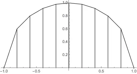
visualTrapezoidRule[Sqrt[1 - #^2] &, -1, 1, 10]

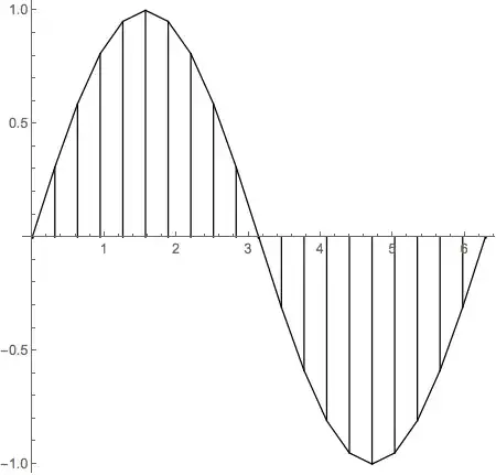
visualTrapezoidRule[Sin, 0, 2 π, 20, 1]

You are very welcoming to new comers with homework. :) – Anton Antonov Jun 11 '17 at 15:54 — Anton Antonov, Jun 11 '17 at 15:54

Visualization of numerical integration

1 Answers1