3D heatmap density plot

Question

I have a set of data that looks like {{x1, y1, z1}, {x2, y2, z2}, ...} so it describes points in 3D space. I want to make a heatmap out of this data. So that points with a high density are shown as a cloud and marked with different colors dependend of the density.

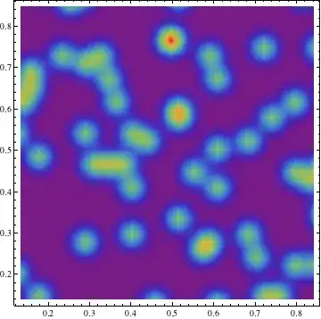
In fact, I want the result of this script just for 3D:

data = RandomReal[1, {100, 2}];
SmoothDensityHistogram[data, 0.02, "PDF", ColorFunction -> "Rainbow", Mesh -> 0]

enter image description here

It is a great example!! for me I used the Image3D function of mathematica 9 but my problem is how I can change the dimensions of each voxel using Image3D[] function. — phdstudent, Oct 04 '13 at 14:49
You should ask a different question, not post your question as an answer. — RunnyKine, Oct 04 '13 at 14:53

score 38 · Accepted Answer · edited Jan 04 '13 at 21:22

If you want to plot a distribution that is three dimensional then first you need to form it! SmoothDensityHistogram plots a smooth kernel histogram of the values $\{x_i,y_i\}$ but as we have three dimensional data here we need the function called SmoothKernelDistribution!

data = RandomReal[1, {1000, 3}];
dist = SmoothKernelDistribution[data];

Now you have got the probability distribution with three variables. So we can simply plot the PDF as a 3d contour plot using ContourPlot3D. Keep in mind that this function is reputed to be little slow.

ContourPlot3D[Evaluate@PDF[dist, {x, y, z}], {x, -2, 2}, {y, -2, 2}, {z, -2, 2}, 
PlotRange -> All, Mesh -> None, MaxRecursion -> 0, PlotPoints -> 160,
ContourStyle -> Opacity[0.45], Mesh -> None, 
ColorFunction -> Function[{x, y, z, f}, ColorData["Rainbow"][z]], 
AxesLabel -> {x, y, z}]

enter image description here

To cut through the contours I used the option!

RegionFunction -> Function[{x, y, z}, x < z || z > y]

In order to check that the data points density is responsible for the shape of the contours we can use Graphics3D

pic = Graphics3D[{ColorData["DarkRainbow"][#[[3]]],
PointSize -> Large, Point[#]} & /@ data, Boxed -> False];
Show[con, pic]

enter image description here

BR

EDIT

To follow up on the 2D example and get warm colours for higher densities

 data = RandomReal[1, {500, 3}];
 dist = SmoothKernelDistribution[data];
 ContourPlot3D[Evaluate@PDF[dist, {x, y, z}], {x, -2, 2}, {y, -2, 2}, 
 {z, -2, 2},PlotRange -> All, Mesh -> None, MaxRecursion -> 0, PlotPoints -> 150, 
  ContourStyle -> Opacity[0.45], Contours -> 5, Mesh -> None,
  ColorFunction -> Function[{x, y, z, f}, ColorData["Rainbow"][f/Max[data]]], 
  AxesLabel -> {x, y, z},
  RegionFunction -> Function[{x, y, z}, x < z || z > y]]

Mathematica graphics

Can't you use ListContourPlot3D, edit nevermind, result is horrible. — s0rce, Jan 04 '13 at 23:07
Great thank you, that script with the edit exactly does the work! One thing if i combine the Point picture with the contour plot i get the following: http://oi47.tinypic.com/34g7otd.jpg I marked the area that is excluded of the contour plot but contains some points ... — norty, Jan 05 '13 at 12:35
@user1936577 please consider to use a simpler user name ;) Now you also need to use same exclusion on your points so that all points are not shown. You can use Cases or Select to pick the relevant points. — PlatoManiac, Jan 05 '13 at 12:44
just changed the name ;) But I want to consider all points in my ContourPlot and now I'm wondering about this area that I marked in the link above — norty, Jan 06 '13 at 09:50

score 20 · Answer 2 · edited Apr 13 '17 at 12:55

The code below (adapted from here) produces an output that is similar to the function Image3D that is unfortunately available only for Mathematica version 9.

Some random 3D data:

data = RandomReal[{-3, 3}, {5000, 3}];

Here we specify the domain to bin (-3, 3) and the binning resolution:

binning = {-3, 3, .5};

The actual code to produce the figure:

binned = BinCounts[data, binning, binning, binning];
dims = Dimensions@binned;
normbinned = N[binned/Max[binned]];
coordswithdataAll = 
  Table[{normbinned[[x, y, z]], {x, y, z}}, {x, 1, dims[[1]]}, {y, 1, 
    dims[[2]]}, {z, 1, dims[[3]]}];
coordswithdata = 
  Table[Select[coordswithdataAll[[j, i]], #[[1]] != 0 &], {j, 
    dims[[1]]}, {i, dims[[1]]}];
cubes = {ColorData["Rainbow"][#1], Opacity@#1, EdgeForm[], 
    Cuboid@#2} &;
output = ParallelMap[cubes @@ # &, coordswithdata, {3}];
Graphics3D[output, PlotRange -> Transpose[{ConstantArray[1, 3], dims + 1}], 
  Lighting -> "Neutral"]

voxels

+1 for being much, much faster than Answer 1. – March Ho Jan 31 '15 at 16:41 — March Ho, Jan 31 '15 at 16:41

3D heatmap density plot

2 Answers2

Linked

Related