I deduce from the little that I know about chemistry that the first ODE (the one whose solution is stored in det) describes the reaction under the assumption of infinite diffusion, i.e., under the assumption that the concentrations at each time instance are constant in the whole medium (I interpret x as time variable here.
If you are going to couple that to a diffusion, then the concentrations have to be functions of both time and space and you will get a system of reaction-diffusion equations, so the equations should look more like this:
xx = {x, y, z};
sx = Sequence @@ xx;
{
  D[r[sx, t], t] == dr Laplacian[r[sx, t], xx] + 0.007 R[sx, t] - 0.2 r[sx, t] L[sx, t],
  D[L[sx, t], t] == dL Laplacian[L[sx, t], xx] + 0.007 R[sx, t] - 0.2 r[sx, t] L[sx, t],
  D[R[sx, t], t] == dR Laplacian[R[sx, t], xx] + 0.2 r[sx, t] L[sx, t] - 0.007 R[sx, t]
 }
with appropriate boundary conditions: an initial condition for each concentration and probably homogeneous Neumann conditions (if you have a closed system).
Here, dr, dL and dR are the diffusivities of the reagents, t is the time variable and {x,y,z} is a three-dimensional space variable. For the one-dimensional case, just use xx = {x}.
If you are looking for the steady state/equilibrium solution, you can drop the dependencies on t and set the left hand sides to 0:
xx = {x, y, z};
sx = Sequence @@ xx;
{
 0 == dr Laplacian[r[sx], xx] + 0.007 R[sx] - 0.2 r[sx] L[sx],
 0 == dL Laplacian[L[sx], xx] + 0.007 R[sx] - 0.2 r[sx] L[sx],
 0 == dR Laplacian[R[sx], xx] + 0.2 r[sx] L[sx] - 0.007 R[sx]
 }
along with boundary conditions of your choice.
So, a complete system with Dirichlet boundary conditions could look like this:
dr = 0.001; dL = 0.001; dR = 0.001;
bc1 = {
   DirichletCondition[r[x] == 0.8, x == 0],
   DirichletCondition[L[x] == 1, x == 0],
   DirichletCondition[R[x] == 0, x == 0],
   DirichletCondition[r[x] == 0, x == 100],
   DirichletCondition[L[x] == 0, x == 100],
   DirichletCondition[R[x] == 0.8, x == 100]
   };
xx = {x};
sx = Sequence @@ xx;
eqn = {
   0 == dr Laplacian[r[sx], xx] + 0.007 R[sx] - 0.2 r[sx] L[sx],
   0 == dL Laplacian[L[sx], xx] + 0.007 R[sx] - 0.2 r[sx] L[sx],
   0 == dR Laplacian[R[sx], xx] + 0.2 r[sx] L[sx] - 0.007 R[sx]
   } ;
sol = NDSolve[Join[eqn, bc1], {r[sx], L[sx], R[sx]}, {x, 0, 100}]
Unfortunately, Mathematica reminds us that NDSolve's FEM solver cannot solve nonlinear PDEs, yet.
A handwoven semi-implicit transient solver (experimental)
First some helper functions
(* Computes load vector for the reaction-diffusion system *)
computeLoad[pat_, celldata_, r_, R_, L_] := cAssembleDenseVector[
   pat,
   Flatten[Join[
     cLoad[celldata, 0.007 R, -0.2 r, L],
     cLoad[celldata, 0.007 R, -0.2 r, L],
     cLoad[celldata, -0.007 R, 0.2 r, L]
     ]],
   {3 Length[r]}
   ];
(* Computes load vector for function (f1 + f2 * f3) *)
cLoad = Block[{PP, P, f1, f2, f3, UU, VV, WW, u, v, w, load},
   PP = Table[CompileGetElement[P, i, 1], {i, 1, 2}]; UU = Table[CompileGetElement[f1, i], {i, 1, 2}];
   VV = Table[CompileGetElement[f2, i], {i, 1, 2}]; WW = Table[CompileGetElement[f3, i], {i, 1, 2}];
   u = t [Function] (1 - t) UU[[1]] + t UU[[2]];
   v = t [Function] (1 - t) VV[[1]] + t VV[[2]];
   w = t [Function] (1 - t) WW[[1]] + t WW[[2]];
   load = Abs[PP[[2]] - PP[[1]]] Integrate[(u[t] + v[t] w[t]) {(1 - t), t}, {t, 0, 1}];
With[{code = N[load]},
    Compile[{{P, _Real, 2}, {f1, _Real, 1}, {f2, _Real, 1}, {f3, _Real, 1}},
     code,
     CompilationTarget -> "C",
     RuntimeAttributes -> {Listable},
     Parallelization -> True,
     RuntimeOptions -> "Speed"
     ]
    ]
   ];
cAssembleDenseVector =
  Compile[{{ilist, _Integer, 1}, {values, _Real, 1}, {dims, _Integer, 1}},
   Block[{A},
    A = Table[0., {i, 1, CompileGetElement[dims, 1]}]; Do[A[[CompileGetElement[ilist, i]]] += Compile`GetElement[values, i], {i, 1, Length[values]}];
    A
    ],
   CompilationTarget -> "C",
   RuntimeAttributes -> {Listable},
   Parallelization -> True,
   RuntimeOptions -> "Speed"
   ];
Next, we intitialize the finite element method and try to use as much built-in capability as possible.
Needs["NDSolve`FEM`"]
ν = 0.01;
dr = ν; dL = ν; dR = ν;
xx = {x};
sx = Sequence @@ xx;
bc = {
   DirichletCondition[r[x] == 0.8, x == 0],
   DirichletCondition[L[x] == 1, x == 0],
   DirichletCondition[R[x] == 0, x == 0],
   DirichletCondition[r[x] == 0, x == 100],
   DirichletCondition[L[x] == 0, x == 100],
   DirichletCondition[R[x] == 0.8, x == 100]
   };
(Initialization of Finite Element Method)
reg = ToElementMesh[
   DiscretizeRegion[Line[{{0}, {100}}]],
   "MeshOrder" -> 1,
   MaxCellMeasure -> 2
   ];
vd = NDSolveVariableData[{"DependentVariables", "Space"} -> {{r, R, L}, {x}}]; sd = NDSolveSolutionData[{"Space"} -> {reg}];
cdata = InitializePDECoefficients[vd, sd,
   "DiffusionCoefficients" -> -DiagonalMatrix[{dr, dR, dL}],
   "MassCoefficients" -> IdentityMatrix[3]
   ("LoadCoefficients"[Rule]{{Sin[2 x]+Cos[x+3 y]}})
   ];
bcdata = InitializeBoundaryConditions[vd, sd, bc];
mdata = InitializePDEMethodData[vd, sd];
(Discretization)
dpde = DiscretizePDE[cdata, mdata, sd];
dbc = DiscretizeBoundaryConditions[bcdata, mdata, sd];
{load, stiffness, damping, mass} = dpde["All"];
DeployBoundaryConditions[{load, stiffness}, dbc];
cells = reg["MeshElements"][[1, 1]];
n = Length[reg["Coordinates"]];
m = Dimensions[cells][[2]];
celldata = Partition[reg["Coordinates"][[Flatten[cells]]], m];
pat = Flatten[Join[cells, cells + n, cells + 2 n]];
Setting up the time integrator. We use $\theta$-method with θ = 0.8 and time stepsize τ = 0.15.
θ = .8;
τ = 0.15;
aplus = mass + (τ θ) stiffness;
DeployBoundaryConditions[{load, aplus}, dbc];
sol = LinearSolve[aplus, Method -> "Banded"];
aminus = mass + τ (1. - θ) stiffness;
DeployBoundaryConditions[{load, aminus}, dbc];
step[u_] := Module[{load},
  load = SparseArray[
    Partition[
     aminus.u +
      computeLoad[pat, celldata, Sequence @@ Partition[u, n]], 1]];
  DeployBoundaryConditions[{load, stiffness}, dbc];
  sol[Flatten[load]]
  ]
Setting up the initial conditions and computing 10000 time iterations.
r0 = 0.2 + 0.1 RandomReal[{-1, 1}, n];
R0 = 0.2 + 0.1 RandomReal[{-1, 1}, n];
L0 = 0.2 + 0.1 RandomReal[{-1, 1}, n];
data = NestList[step, Join[r0, R0, L0], 10000];
{rlist, Rlist, Llist} = Partition[data, {Length[data], n}][[1]];
A plot of the solutions
Manipulate[
 ListLinePlot[{rlist[[i]], Rlist[[i]], Llist[[i]]},
  PlotRange -> {-1, 1} 4,
  PlotLegends -> {"r", "R", "L"},
  AxesLabel -> {"x", "Concentration"}
  ],
 {i, 1, Length[rlist], 1}
 ]
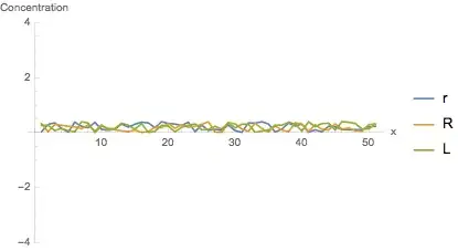
The result is somewhat odd. I guess something must be wrong about the reaction part of the equations... (Of course, bugs can be also contained in other parts.)