1

I know that Mathematica can solve a PDE numerically, but I wonder if it is possible to obtain the exact solution. For example, consider the heat equation

$$u_t = \kappa u_{xx} $$

Is it possible to solve it with a set of initial and boundary conditions to calculate the exact equation of $u$

$$u = f(x,t)$$ and $$u(x=0) = f(t)$$

I don't need numeral solution or the graph but the general equations.

EXAMPLE

One dimensional heat flow in an slab, one side is insulated and the other side at a constant flux of heat

$$ u(x,0) = U\\ u_x(0,t) = 0\\ u_x(L,t) = T $$

The solution is available from the textbooks. I just wonder, if Mathematica can give us the solution, as we can slightly alter the conditions to find new solutions.

Kiera
  • 11
  • 2
  • 3
    That depends really on the domain. For example, the fundamental solution for the disk is known and the symbolic solution can be obtained via convolution with it. – Henrik Schumacher Aug 07 '18 at 11:32
  • @HenrikSchumacher I am interested in the boundary conditions rather than domain. I would consider one-dimensional. It may seem strange, but I am interested to find the solution by Laplance transformation or so. I add an example. – Kiera Aug 07 '18 at 11:45
  • Welcome to Mma.SE. Start by taking the [tour] now and learning about asking and what's on-topic. Always [edit] if improvable, show due diligence, and be specific, include minimal working example of code and data you have tried in formatted form. By doing all this you help us to help you and likely you will inspire great answers. The site depends on participation, as you receive give back: vote and answer questions, keep the site useful, be kind, correct mistakes and share what you have learned. – rhermans Aug 07 '18 at 13:57

2 Answers2

5

Sometimes you can solve pde's symbollically.

example heat equation:

DSolve[{Derivative[0, 1][u][x, t] == Derivative[2, 0][u][x, t],u[0, t] == f[t]}, u, {x, t}][[1]]
Ulrich Neumann
  • 53,729
  • 2
  • 23
  • 55
4

The specific example can be solved with the help of finite Fourier cosine transform and its inversion:

With[{u = u[t, x]},
 eq = D[u, t] == κ D[u, x, x];
 ic = u == U[x] /. t -> 0;
 bc = {D[u, x] == 0 /. x -> 0, D[u, x] == T /. x -> L};]

Format@finiteFourierSinTransform[f_, __] := Subscript[ℱ, s][f]
Format@finiteFourierCosTransform[f_, __] := Subscript[ℱ, c][f]

help[index_] := 
 Module[{tset = 
    finiteFourierCosTransform[{eq, ic}, {x, 0, L}, index] /. Rule @@@ bc /. 
     HoldPattern@finiteFourierCosTransform[f_ /; ! FreeQ[f, u], __] :> f},
  tsol = DSolve[tset, u[t, x], t][[1, 1, -1]]]

tsolgeneral = help[n]

tsolzero = help[0]

tsolfunc[n_] = Piecewise[{{tsolgeneral, n != 0}}, tsolzero]

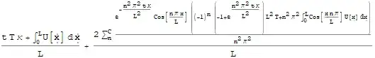
sol = inverseFiniteFourierCosTransform[tsolfunc[n], n, {x, 0, L}] // transformToIntegrate

Mathematica graphics

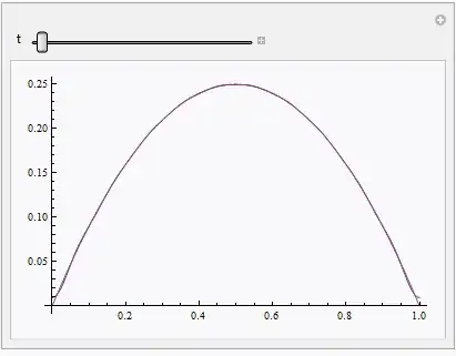
Let's check the solution numerically with $U=x(1-x),\ L=1,\ κ = 1,\ T = 1$:

U = (# (1 - #) &); L = 1; κ = 1; T = 1;
nsol = NDSolveValue[{eq, ic, bc}, u, {t, 0, 1/10}, {x, 0, 1}, 
   Method -> {"MethodOfLines", 
     "DifferentiateBoundaryConditions" -> {True, "ScaleFactor" -> 5000}}];

With[{expr = 
   Block[{C = 20, HoldForm = Identity, 
     Sum = Function[{expr, lst}, Total@Table[expr, lst], HoldAll]}, sol]}, 
 Manipulate[Plot[{expr, nsol[t, x]}, {x, 0, 1}, PlotRange -> All], {t, 0, 1/10}]]
Clear[U, L, κ, T]

enter image description here

Remark

  1. Finite Fourier Cosine transform at $n=0$ is calculated separately here because currently finiteFourierCosTransform cannot handle the singularity at $n=0$ properly.

  2. The reason why "DifferentiateBoundaryConditions" option is added is explained in this post.

xzczd
  • 65,995
  • 9
  • 163
  • 468
  • don't you get the error, NDSolveValue::ibcinc: Warning: boundary and initial conditions are inconsistent.? – Googlebot Aug 07 '18 at 20:34
  • @Googlebot It doesn't matter as long as "DifferentiateBoundaryConditions" option is properly set. For more information you can check the last link in my answer. – xzczd Aug 07 '18 at 23:38