Implement finite Fourier transforms

Question

Recently I came across finite Fourier transforms, which can be used for solving certain type of boundary value problem (BVP) of linear partial differential equation (PDE) with constant coefficient. The definition of the transforms and their properties are as follows.

Finite Fourier sine transform and its inversion:

$$\mathcal{F}_s \{f (x)\}=\tilde{f}_s(n)=\int_0^a f (x) \sin (\frac{n\pi x}{a}) \, dx$$ $$\mathcal{F}^{-1}_s \{\tilde{f}_s(n)\}=f (x)=\frac{2}{a} \sum _{n=1}^{\infty } \tilde{f}_s(n) \sin (\frac{n \pi x}{a}) $$

Finite Fourier cosine transform and its inversion:

$$\mathcal{F}_c \{f (x)\}=\tilde{f}_c(n)=\int_0^a f (x) \cos (\frac{n\pi x}{a}) \, dx$$ $$\mathcal{F}^{-1}_c \{\tilde{f}_c(n)\}=f (x)=\frac{1}{a}\tilde{f}_c(0)+\frac{2}{a} \sum _{n=1}^{\infty } \tilde{f}_c(n) \cos (\frac{n \pi x}{a}) $$

Their main properties playing role in PDE solving are:

$$\mathcal{F}_s \{f' (x)\}=-(\frac{n \pi}{a})\tilde{f}_c(n)$$ $$\mathcal{F}_c \{f' (x)\}=(\frac{n \pi}{a})\tilde{f}_s(n)+(-1)^{n}f'(a)-f'(0)$$

For more information you can refer to this material or Chapter 10 of this book.

Can we implement these transforms in Mathematica?

Answer 1

This post contains several code blocks, you can copy them easily with the help of importCode.

---

The following is my implementation for finite Fourier transforms. Here I've also implemented finite Fourier transform, which can be viewed as the counterpart of FourierSeries:

ClearAll[finiteFourierSinTransform, finiteFourierCosTransform, finiteFourierTransform, 
transformToIntegrate]
(#[(h : List | Plus | Equal)[a__], x_, n_] := Function[f, #[f, x, n]] /@ h[a];
    #[a_ b_, {x_, xmin_, xmax_}, n_] /; FreeQ[b, x] := 
     b #[a, {x, xmin, xmax}, n]) & /@ {finiteFourierSinTransform, 
   finiteFourierCosTransform, finiteFourierTransform};
argumentPattern = (#[
      Derivative[i___, j_, k___][head_][var1___, x_, var2___], {x_, xmin_, xmax_}, n_] /;
      Length@{i} === Length@{var1} && j > 0) &;
With[{f = Derivative[i, j - 1, k][head]},
 Evaluate@argumentPattern@
    finiteFourierSinTransform := -((n Pi)/(xmax - xmin)) finiteFourierCosTransform[
    f[var1, x, var2], {x, xmin, xmax}, n];
Evaluate@argumentPattern@
    finiteFourierCosTransform := ((n Pi)/(xmax - xmin)) finiteFourierSinTransform[
     f[var1, x, var2], {x, xmin, xmax}, n] + (-1)^n f[var1, xmax, var2] - 
   f[var1, xmin, var2];
Evaluate@argumentPattern@
    finiteFourierTransform := ((2 I n Pi)/(xmax - xmin)) finiteFourierTransform[
     f[var1, x, var2], {x, xmin, xmax}, 
     n] + (-1)^-n (f[var1, xmax, var2] - f[var1, xmin, var2]);
(#[f_ /; AtomQ@f || Quiet@Context@Evaluate@Head[f] === "System`", {x_, xmin_, xmax_}, 
      n_] :=
     With[{assump = {n ∈ Integers, xmax > xmin, #3}, 
       integral = 
        Function[index, 
         Simplify@Integrate[f #2[(index Pi (x - xmin))/(xmax - xmin)], {x, xmin, xmax}]]},
      Module[{general =
         Assuming[assump, integral@n]}, 
       With[{singularity = 
          If[IntegerQ@n, {}, 
           Union@Join[If[#2 === Cos, {0}, {}], 
             Piecewise[{{{}, # === n}}, #] &@(n /. 
                Solve[Flatten@{assump, Denominator@Together@general == 0}, n])]]},
        Piecewise[{integral@#, n == #} & /@ singularity, general]]
       ]
      ]) & @@@ {{finiteFourierSinTransform, Sin, n > 0}, {finiteFourierCosTransform, Cos,
     n >= 0}};
finiteFourierTransform[
   f_ /; AtomQ@f || Quiet@Context@Evaluate@Head[f] === "System`", {x_, xmin_, xmax_}, 
   n_] :=
  With[{assump = {n ∈ Integers, xmax > xmin}, 
    integral = Function[index, 
      Simplify@Integrate[
        f E^(-((2 I index π (x - xmin - (xmax - xmin)/2))/(xmax - xmin))), {x, xmin, 
         xmax}]]},
   Module[{general =
      Assuming[assump, integral@n]}, 
    With[{singularity = 
       If[IntegerQ@n, {}, 
        Piecewise[{{{}, # === n}}, #] &@(n /. 
           Solve[Flatten@{assump, Denominator@Together@general == 0}, n])]},
     Piecewise[{integral@#, n == #} & /@ singularity, general]]
    ]
   ]
 ]
inverseFiniteFourierSinTransform[f_, n_, {x_, xmin_, xmax_}] := 
 2/(xmax - xmin) HoldForm@Sum[#, {n, C}] &[f Sin[(n Pi (x - xmin))/(xmax - xmin)]]
inverseFiniteFourierCosTransform[f_, n_, {x_, xmin_, xmax_}] := 
 1/(xmax - xmin) (f /. n -> 0) + 2/(xmax - xmin) HoldForm@Sum[#, {n, C}] &@
  Simplify[f Cos[(n Pi (x - xmin))/(xmax - xmin)], n > 0]
inverseFiniteFourierTransform[f_, n_, {x_, xmin_, xmax_}, Re] := 
 1/(xmax - xmin) ((f E^((2 I n π (x - xmin - (xmax - xmin)/2))/(xmax - xmin)) /. 
        n -> 0) + 2 HoldForm@Sum[#, {n, 1, C}] &@
    Simplify[f E^((2 I n π (x - xmin - (xmax - xmin)/2))/(xmax - xmin)) // Re, 
     n ∈ Integers])
inverseFiniteFourierTransform[f_, n_, {x_, xmin_, xmax_}] := 
 1/(xmax - xmin) (HoldForm@Sum[#, {n, -C, C}] &@
    Simplify[f E^((2 I n π (x - xmin - (xmax - xmin)/2))/(xmax - xmin)), 
     n ∈ Integers])
transformToIntegrate[expr_] := 
  expr /. (HoldPattern@#[f_, {x_, xmin_, xmax_}, n_] :> 
        RuleCondition@(HoldForm@Integrate[#, {[FormalX], xmin, xmax}] &)[
          f #2[(n Pi (x - xmin))/(xmax - xmin)] /. 
           x -> [FormalX]] & @@@ {{finiteFourierSinTransform, 
        Sin}, {finiteFourierCosTransform, Cos}}) /. 
   HoldPattern@finiteFourierTransform[f_, {x_, xmin_, xmax_}, n_] :> 
    RuleCondition@(HoldForm@Integrate[#, {[FormalX], xmin, xmax}] &)@
      Simplify[f E^(-((2 I n π (x - xmin - (xmax - xmin)/2))/(xmax - xmin))) /. 
        x -> [FormalX], n ∈ Integers];

I'm still in v9 so choose HoldForm rather than Inactivate to hold the expression.

Example

Here I'll show the usage of these functions by solving the following initial-boundary value problem (IBVP) which, as far as I can tell, can't be handled by DSolve at the moment:

$$u_{t}=\kappa u_{xx}\,, \ \ \ \ \ 0 \leq x \leq a\,,\ \ t>0$$ $$u(0,t)=0=u(a,t)$$ $$u(x,0)=f(x)\ \ \text{for}\ 0 \leq x \leq a$$

First, interprete the equation to Mathematica code:

With[{u = u[t, x]}, eq = D[u, t] == k D[u, x, x];
 ic = {u == f[x] /. t -> 0};
 bc = u == 0 /. {{x -> 0}, {x -> a}};]

Then, use finite Fourier sine transform to eliminate the derivative with respect to $x$. I've used Format to make the output better looking:

Format@finiteFourierSinTransform[f_, __] := Subscript[\[ScriptCapitalF], s][f]
Format@finiteFourierCosTransform[f_, __] := Subscript[\[ScriptCapitalF], c][f]
finiteFourierSinTransform[{eq, ic}, {x, 0, a}, n]

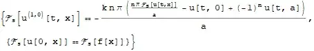
The transformed system involves u[t, 0] and u[t, a]: they're the boundary condition (b.c.) at hand! So, plug them in:

% /. Rule @@@ bc

Now the equation becomes an ordinary differential equation (ODE), which can be solved with DSolve:

tset = % /. HoldPattern@finiteFourierSinTransform[f_ /; ! FreeQ[f, u], __] :> f
tsol = DSolve[tset, u[t, x], t][[1, 1, -1]]

Remark

Notice I've stripped off finiteFourierSinTransform before solving the ODE because DSolve has difficulty in understanding expression like finiteFourierSinTransform[u[t, x], {x, 0, a}, n]. Just remember that u[t, x] actually denotes finiteFourierSinTransform[u[t, x], {x, 0, a}, n] in tset.

The last step is to transform back. You can use transformToIntegrate to make finiteFourierSinTransform denote as an integration:

sol = inverseFiniteFourierSinTransform[tsol, n, {x, 0, a}] // transformToIntegrate

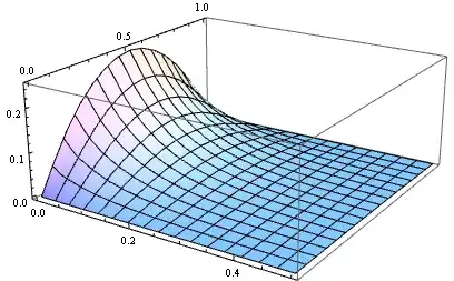
The following is the resulting graph by taking the first 5 terms of the series and choosing $f(x) = x (1 - x), a = 1, \kappa = 1$:

Plot3D[Block[{C = 5, f = (# (1 - #) &), a = 1, k = 1, HoldForm = Identity, 
    Sum = Function[{expr, lst}, Total@Table[expr, lst], HoldAll] }, sol] // Evaluate, {t,
   0, 1/2}, {x, 0, 1}, PlotRange -> All]

Possible issues

1. These functions are built on Solve, Integrate, etc. so they inherit all their limitations.

2. The singularity test is simple and crude so it will probably fail in complicated cases.

3. The transforms are only suitable for certain types of BVP and IBVP. A typical troublesome case is the 5th exercise in Chapter 10 of Lokenath Debnath's book:

$$u_{t}=\kappa u_{xx}\,, \ \ \ \ \ 0 \leq x \leq a\,,\ \ t>0$$ $$u_{x}(0,t)=f(t)$$ $$u_{x}(a,t)+h u(a,t)=0$$ $$u(x,0)=0\ \ \text{for}\ 0 \leq x \leq a$$

For this exercise Lokenath has given the following hint:

Hint: $$\tilde{f}_s(n)=\int_0^a f (x) \sin (\xi_{n}x) \, dx$$ $$f(x)=\mathcal{F}_s^{-1} \{\tilde{f}_s(n)\}=\frac{2}{a}\sum _{n=0}^{\infty}\frac{(h^2+\xi_n^2)\tilde{f}_s(n)\sin(x \xi_n)}{h+(h^2+\xi_n^2)}$$ where $\xi_n$ is the root of the equation $\xi \cot(a \xi)+h=0$. $$u(x,t)=(\frac{2}{a})\sum _{n=1}^{\infty }\frac{\xi_n(h^2+\xi_n^2)}{h+(h^2+\xi_n^2)}\int_0^t f (\xi)\exp[-\kappa \xi_n(t-\xi)]\sin(x \xi_n)\, d\xi$$

The $\tilde{f}_s(n)$ is a general finite Fourier sine transform. (This paper is a possible reference. ) I might implement these transforms someday.