5

Follow from the discussion 2D+1 PDE problem

$\partial_t u(t,x,y)=-y\partial_{x}u+\partial_{y}\left[γ(1+sin(3x)) yu+A sin(3x)u+γkT(1+sin(3x))\partial_{y}u\right]$

with $u(0,x,y)=\frac{1}{2\pi}e^{-(x^2+y^2)/2}$

and periodic boundary condition:

$u(t,-\pi,y)=u(t,\pi,y)$

In $y$-direction, it is unbounded.

The code and result are shown below

a = 1;
T = 50;
ωb = -5; ωt = 5;
A = 1;
γ = .1;
kT = 0.1;
φ = 0;
mol[n_Integer, o_: "Pseudospectral"] := {"MethodOfLines", 
  "SpatialDiscretization" -> {"TensorProductGrid", "MaxPoints" -> n, 
    "MinPoints" -> n, "DifferenceOrder" -> o}}

With[{u = u[t,θ, ω]}, 
 eq = D[u, t] == -D[ω u,θ] - 
     D[-A Sin[3θ] u, ω] + γ (1 + 
        Sin[3θ])  kT  D[
       u, {ω, 2}] + γ  (1 + 
        Sin[3θ]) D[ω u, ω];
ic = u == E^(-((ω^2 +θ^2)/(2 a^2))) 1/(2 π a) /. 
    t -> 0];
ufun = NDSolveValue[{eq, ic, 
     u[t, -π, ω] == u[t, π, ω], 
     u[t,θ, ωb] == 0, u[t,θ, ωt] == 0}, 
    u, {t, 0, 
     T}, {θ, -π, π}, {ω, ωb, ωt}, 
    Method -> mol[35], MaxSteps -> Infinity]; // AbsoluteTiming
plots = Table[
    Plot3D[Abs[
      ufun[t,θ, ω]], {θ, -π, π}, {
ω, ωb, ωt}, AxesLabel -> Automatic, 
     PlotPoints -> 30, BoxRatios -> {Pi, ωb, 1}, 
     ColorFunction -> "LakeColors", PlotRange -> All], {t, 0, T, 
     1}]; // AbsoluteTiming
ListAnimate[plots]

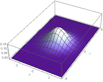
enter image description here

The problem is if we increase the coefficient $A$ then the program is no longer stable. Simply refine the grid points are still not able to solve the problem entirely. Perhaps there is a smarter way to sample the grid points and time step, or?

Result for $A=2$:

enter image description here

It's crazy..

Btw, since the x-direction is periodic but y is not, is it possible to use pseudospectral in x and keep the default setting for y?

Update (8/22)

Increasing A to 3 with MaxPoints=71 and MinPoints=51 still fails to converge. But my friend he can solve A=8 by Julia code with much fewer points less than a minute. There must be something wrong for my grids...

Note: The function u should be localized in 3 minima of potential $-\cos{3\theta}$. enter image description here

Bob Lin
  • 445
  • 2
  • 8
  • Can be used mol[n_Integer, o_: "Pseudospectral"] := {"MethodOfLines", "SpatialDiscretization" -> {"TensorProductGrid", "MaxPoints" -> 2*n, "MinPoints" -> n, "DifferenceOrder" -> o}} – Alex Trounev Aug 22 '18 at 02:01
  • 2
    As to the update: Notice the difference scheme may have significant influence on the performance, here is an example. You'd better ask your friend what difference scheme is used by him. – xzczd Aug 22 '18 at 09:11

1 Answers1

8

It is necessary to increase the option "MaxPoints", for example, twice:

a = 1;
T = 50;
ωb = -5; ωt = 5;
A = 2;
γ = .1;
kT = 0.1;
φ = 0;
mol[n_Integer, o_: "Pseudospectral"] := {"MethodOfLines", 
  "SpatialDiscretization" -> {"TensorProductGrid", "MaxPoints" -> 2*n,
     "MinPoints" -> n, "DifferenceOrder" -> o}}

With[{u = u[t, θ, ω]}, 
  eq = D[u, t] == -D[ω u, θ] - D[-A Sin[3 θ] u, ω] + γ (1 + Sin[3 θ]) kT D[u, {ω, 2}] + γ (1 + Sin[3 θ]) D[ω u, ω];
  ic = u == E^(-((ω^2 + θ^2)/(2 a^2))) 1/(2 π a) /. 
    t -> 0];
ufun = NDSolveValue[{eq, ic, 
     u[t, -π, ω] == u[t, π, ω], 
     u[t, θ, ωb] == 0, u[t, θ, ωt] == 0}, 
    u, {t, 0, 
     T}, {θ, -π, π}, {ω, ωb, ωt}, 
    Method -> mol[35], MaxSteps -> Infinity]; // AbsoluteTiming
plots = Table[
    Plot3D[Abs[
      ufun[t, θ, ω]], {θ, -π, π}, {ω, ωb, ωt}, AxesLabel -> Automatic, 
     PlotPoints -> 30, BoxRatios -> {Pi, ωb, 1}, 
     ColorFunction -> "LakeColors", PlotRange -> All], {t, 0, T, 
     1}]; // AbsoluteTiming
ListAnimate[plots]

fig1

I give two tips on how to shorten the integration time by a factor of 10 and get rid of the large parameter A. First, we must divide all the terms of the equation into A. Secondly, we need to make the substitution t->T*t. Then the integration is always carried out on the interval (0,1), and the large parameter TA just normalizes the time derivative. We now make the normalization to gamma, then the divergence is completely eliminated. In addition, we need to add a new parameter q<<1 to exclude the degeneracy of the equation at the line $\sin (3\theta 0=-1).

K = 35; a = 1;
T = 1;
ωb = -5; ωt = 5;
A = 8;
γ = .1;
T0 = 50*A*γ;
kT = 0.1;
φ = 0;
q = 10^-5;
mol[n_Integer, o_: "Pseudospectral"] := {"MethodOfLines", 
  "SpatialDiscretization" -> {
   "TensorProductGrid", 
   "MaxPoints" -> 2*n, 
   "MinPoints" -> n, 
   "DifferenceOrder" -> o
   }
  };

With[{u = u[t, θ, ω]}, 
  eq = D[u, t]/T0 == -D[ω u, θ]/A/γ - D[-Sin[3 θ] u, ω]/γ + (1 + q*Sin[3 θ]) kT D[u, {ω, 2}] + (1 + q*Sin[3 θ]) D[ω u, ω];
  ic = u == E^(-((ω^2 + θ^2)/(2 a^2))) 1/(2 π a) /.  t -> 0
  ];
ufun = NDSolveValue[{eq, ic, 
     u[t, -π, ω] == u[t, π, ω], 
     u[t, θ, ωb] == 0, u[t, θ, ωt] == 0}, 
    u, {t, 0, 
     T}, {θ, -π, π}, {ω, ωb, ωt}, 
    Method -> mol[K], MaxSteps -> Infinity]; // AbsoluteTiming
plots = Table[
    Plot3D[Abs[
      ufun[t, θ, ω]], {θ, -π, π}, {ω, ωb, ωt}, 
      AxesLabel -> Automatic, 
      PlotPoints -> 30, ColorFunction -> "LakeColors", 
      PlotRange -> All
      ], 
     {t, 0, T, .1*T}]; // AbsoluteTiming
ListAnimate[plots]

fig2

Henrik Schumacher
  • 106,770
  • 7
  • 179
  • 309
Alex Trounev
  • 44,369
  • 3
  • 48
  • 106
  • 1
    Just a side note: by checking ufun["Grid"] // Dimensions one can figure out NDSolve has actually chosen Method -> {"MethodOfLines", "SpatialDiscretization" -> {"TensorProductGrid", "MaxPoints" -> {71, 35}, "MinPoints" -> {71, 35}, "DifferenceOrder" -> "Pseudospectral"}}. – xzczd Aug 22 '18 at 03:11
  • Note that giving different values for options "MaxPoints", "MinPoints" allows us to stabilize the solution in different tasks. – Alex Trounev Aug 22 '18 at 03:53
  • According to my personal experience, in certain cases allowing NDSolve to determine grid size by itself seems to make things worse. (This may be caused by the relatively coarse priori error estimate. ) That's the reason why I prefer making MinPoints and MaxPoints the same. But anyway, the priori error estimate does do a good job in this case, I'm impressed. – xzczd Aug 22 '18 at 04:21
  • Many thanks for your suggestion! is it possible to use difference order->Pseudopectral in x-direction only to avoid additional computational effort? Does keeping increase A imply large MaxPoints (e.g. A=8)? – Bob Lin Aug 22 '18 at 05:46
  • Unfortunately, I just try MaxPoints=71 and MinPoints=35 for A=8. It takes a minute to run the program but eventually it becomes unstable still. – Bob Lin Aug 22 '18 at 06:20
  • Is the rule of thumb just increasing the MaxPoints? – Bob Lin Aug 22 '18 at 06:26
  • @Bob Lin See the new code for this case – Alex Trounev Aug 22 '18 at 09:26
  • Very good! But there are some messy behavior in the boundary? – Bob Lin Aug 22 '18 at 10:48
  • @AlexTrounev I would like to see the result for A=8 and T=50. Just wondering if it is stable. – Bob Lin Aug 22 '18 at 10:51
  • @Bob Lin Fig. 2 this is the case A = 8, T = 50. It is quite stable. – Alex Trounev Aug 22 '18 at 10:56
  • Okay, now I see. But why q=10^-5? Would this change the problem? – Bob Lin Aug 22 '18 at 11:06
  • Also, I suppose the result in the Fig.2 should be the pretty much the same as A=1 probably. – Bob Lin Aug 22 '18 at 11:08
  • In your model, the coefficients of the highest derivatives are 0 at the boundaries, i.e. the equation is degenerate. To avoid this, in numerical calculations, we must step back from zero. This eliminates the instability. The parameter q allows you to see how the instability is eliminated. – Alex Trounev Aug 22 '18 at 11:19
  • The coefficients go to zero on the lines $\sin (3\theta )=-1$ – Alex Trounev Aug 22 '18 at 11:33
  • I set your code from T=50 to T=300. Also, I increase MaxPoints but still not able to reach the figure like A=1. Is it due to that the initial condition is hard to solve? – Bob Lin Aug 22 '18 at 11:45
  • We are already at the limit of the length of the discussion. I changed the code. Now it works longer, but it is stable even in the original boundaries (-5,5) – Alex Trounev Aug 22 '18 at 11:53
  • @AlexTrounev I add the note for the expected result. In the end, there should be only 3 nice smooth peaks at t->infinity. – Bob Lin Aug 22 '18 at 12:35
  • @AlexTrounev I would say your result is correct initially, but in the end it has some numerical problem. – Bob Lin Aug 22 '18 at 13:15