It is possible that the condition of periodicity 'u[t, -π] == u[t, π]' is wrong. A solution with such a potential cannot be symmetric about zero. On the other hand, we do not know which method to solve is correct. We can compare solutions
sol = NDSolveValue[{I D[u[t, x], t] == -D[u[t, x], {x, 2}] +
     I Sin[x] u[t, x], u[0, x] == Exp[-(x - Pi)^2] Exp[I (x - Pi)],
   PeriodicBoundaryCondition[u[t, x], x == 2*\[Pi],
    Function[x, x - 2*\[Pi]]]}, u, {t, 0, 5}, {x, 0, 2*Pi}];
sol1 = NDSolveValue[{D[u[t, x], t] ==
    I*D[u[t, x], {x, 2}] + Sin[x] u[t, x],
   u[0, x] == Exp[-(x - Pi)^2] Exp[I (x - Pi)],
   u[t, 0] == u[t, 2*\[Pi]]}, u, {t, 0, 5}, {x, 0, 2*\[Pi]},
  Method -> {"MethodOfLines",
    "SpatialDiscretization" -> {"TensorProductGrid",
      "MaxPoints" -> 10000}}];
sol2 = NDSolveValue[{I D[u[t, x], t] == -D[u[t, x], {x, 2}] +
     I Sin[x] u[t, x], u[0, x] == Exp[-(x - Pi)^2] Exp[I (x - Pi)],
   u[t, 0] == u[t, 2*\[Pi]]}, u, {t, 0, 5}, {x, 0, 2*\[Pi]},
  Method -> {"MethodOfLines",
    "SpatialDiscretization" -> {"TensorProductGrid",
      "MaxPoints" -> 100}}]
    {DensityPlot[Abs[sol[t, x]], {x, 0, 2*Pi}, {t, 0, 5},
      PlotPoints -> 50, MaxRecursion -> 2, PlotLegends -> Automatic,
      ColorFunction -> Hue, FrameLabel -> {"x", "t"}, PlotRange -> All],
     DensityPlot[Abs[sol1[t, x]], {x, 0, 2*Pi}, {t, 0, 5},
      PlotPoints -> 50, MaxRecursion -> 2, PlotLegends -> Automatic,
      ColorFunction -> Hue, FrameLabel -> {"x", "t"}, PlotRange -> All],
     DensityPlot[Abs[sol1[t, x]], {x, 0, 2*Pi}, {t, 0, 5},
      PlotPoints -> 50, MaxRecursion -> 2, PlotLegends -> Automatic,
      ColorFunction -> Hue, FrameLabel -> {"x", "t"}, PlotRange -> All]}
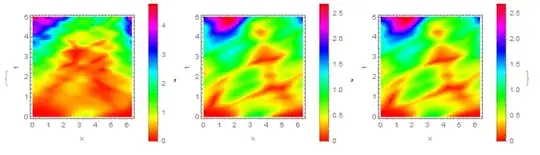
Obviously, one of the methods is erroneous. But only sol1 and sol2 have a message NDSolveValue::mxsst: Using maximum number of grid points 10000 allowed by the MaxPoints or MinStepSize options for independent variable x. and NDSolveValue::mxsst: Using maximum number of grid points 100 allowed by the MaxPoints or MinStepSize options for independent variable x.


Iin front of the potential? – Dec 17 '18 at 13:12\[Psi] = NDSolve[{ D[u[t, x], t] == I*D[u[t, x], {x, 2}] + Sin[x] u[t, x], u[0, x] == Exp[-x^2] Exp[I x], u[t, -\[Pi]] == u[t, \[Pi]]}, u, {t, 0, 5}, {x, -\[Pi], \[Pi]}, Method -> {"MethodOfLines", "SpatialDiscretization" -> {"TensorProductGrid", "MaxPoints" -> 101}}]Then it plots something. – Dec 17 '18 at 13:18Method -> "MethodOfLines"toNDSolve. It took a few minutes though. – Alexei Boulbitch Dec 18 '18 at 09:00