Plot a 2D vector path onto a surface

Question

In my calculus 3 course, we're studying gradients and have a project that takes a combination of 3D Gaussian radial surfaces and a basic parametric path $r(t) = \{x(t),y(t)\}$ to see how the gradient changes and so forth with respect to the coordinates of $r(t)$ on the path. I need to figure out a way to plot the surface and path together. I've got both of them figured out, just can't combine them. Any ideas?

So here's what I have so far: 6 Gaussian radials $\lambda e^{-(\epsilon r)^2}$ where $r=||x-x_i||.$ All six are added up to form a "mountain range". A group of hikers are hiking the path

$$r(t)=(2.5 + 1.8 \sin(4t),2 - 1.2 \cos(4 t))$$

which is just a simple ellipse.

I'm trying to figure out a way to "lay" the path on the surface.

Answer 1

Some programming principles help us make short work of this. The key principle is to encapsulate what's going on.

First, the surface. It depends on some parameters, so let's be explicit about that, rather than letting those parameters run around loose as "global" variables. To illustrate, I begin by generating some (reproducible) random values for these parameters:

n = 6;
SeedRandom[17];
λ = RandomReal[GammaDistribution[4, 1/5], n];
ϵ = RandomReal[GammaDistribution[3, 1/4], n];
x0 = RandomVariate[BinormalDistribution[{2.5, 2}, {2, 1}, 1/2], n];

I am going to change the meaning of the $\epsilon$ a little, though: it is more natural that they be proportional to the widths of the "hills," so they will appear in the denominator below. Here is the "Gaussian radial" function:

f[x_, {λ_, ϵ_, x0_}] := Sum[λ[[i]] Exp[-(Norm[x - x0[[i]]]/ϵ[[i]])^2], {i, 1, Length[λ]}];

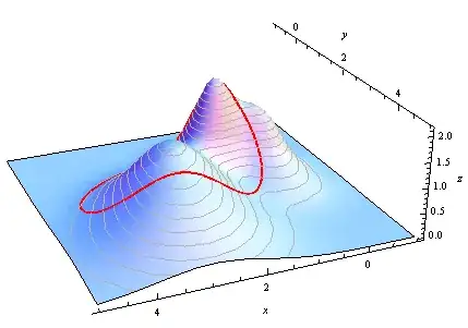
Its first argument is an $(x,y)$ coordinate pair and its second is a list of the parameters. It computes the topographic elevation at $(x,y)$ by summing the values of the Gaussians at $(x,y)$. We can make a pretty pseudo-3D plot of the topography (and store it in a variable for later display):

dem = Plot3D[
  f[{x, y}, {λ, ϵ, x0}], {x, -1, 5}, {y, -1, 5}, PlotRange -> {Full, Full, Full},
    PlotStyle -> Opacity[0.9], MeshFunctions -> {#3 &}, MeshStyle -> GrayLevel[0.7]]

Second, the key Calculus idea is that the hikers' path is parameterized by their base curve $t\to \gamma(t) = (x(t), y(t))$; it merely needs to be "lifted" to the proper height given by $f(\gamma(t), \ldots)$. (The dots represent values of the parameters controlling the shape of $f$.) The fully parameterized hike therefore is

$$t \to (x(t), y(t), f((x(t), y(t)), \ldots)).$$

Because we have encapsulated the key functionality, this is easy and straightforward to code:

γ[t_] := {5/2, 2} + {9 Sin[4 t], -6 Cos[4 t]}/5;
path[t_, {λ_, ϵ_, x0_}] := With[{x = γ[t]}, Append[x, f[x,  {λ, ϵ, x0}]]];

(For a general-purpose solution you might want to make γ and f arguments of path, too, in keeping with the idea that everything a function like path depends on should be explicitly exhibited, within reason.)

ParametricPlot3D takes care of the graphical display:

hike = ParametricPlot3D[path[t, {λ, ϵ, x0}], {t, 0, π/2}, PlotStyle -> Directive[Thick, Red]];

Finally, use Show to assemble the plots of the surface and the path and control the final appearance:

Show[dem, hike, Boxed -> False, BoxRatios -> Automatic, AxesLabel -> {x, y, z}]

Edit

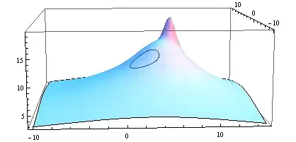
If you wish to study the hike in more detail, you may introduce a second parameter to path to fill it in vertically: let it multiply the $z$ value and range from $0$ to $1$. I will leave the implementation as an exercise and just show the result:

This also shows how the technique is capable of accurately drawing a hike which is not a closed loop.

Answer 2

f[{a_, b_, r0 : {x0_, y0_}}, r : {x_, y_}] := a Exp[-(b Norm[r - r0])^2];
a = Range@6;
b = (1/Reverse@Range@6)^2;
r0 = Array[{#, #} &, 6];

u[{x_, y_}] := Total[f[#, {x, y}] & /@ Transpose@{a, b, r0}]
p[t_] := {2.5 + 1.8 Sin@(4 t), 2 - 1.2 Cos[4 t]}
Show[Plot3D[u[{x, y}], {x, -10, 15}, {y, -10, 15}, Mesh -> False], 
     ParametricPlot3D[Flatten[{p[t], u[p[t]]}], {t, 0, 2 Pi}]]

Edit

Another possible plot:

Show[
 Plot3D[u[{x, y}], {x, -10, 15}, {y, -10, 15}, 
  PlotStyle ->Directive[Orange,Opacity[.95],Specularity[White, 10]],MeshFunctions -> {#3 &}],
 ParametricPlot3D[Flatten[{p[t], z}], {t, 0, 2 Pi}, {z, 0, 20}, Mesh -> None, 
                  PlotStyle -> Directive[Blue, Opacity[.2]]], 
 ParametricPlot3D[Flatten[{p[t], u[p[t]]}], {t, 0, 2 Pi}, PlotStyle-> Directive[Thick, Red]],
 ParametricPlot3D[Flatten[{p[t], 19.8}], {t, 0, 2 Pi}, PlotStyle -> Directive[Thick, Red]]]

Answer 3

Silvia beat me to using MeshFunctions, but here's another way to use it. Similarly it works for this path, but not arbitrary paths, like some of the others.

f = Sum[i j E^(-4 ((x - i)^2 + (y - j)^2)), {i, 1, 4}, {j, 1, 3}];
Plot3D[f, {x, 0, 5}, {y, 0, 4}, Mesh -> {{0}}, 
 MeshFunctions -> 
  Function[{x, y, z}, 
   Evaluate[Subtract @@ 
     Quiet@Eliminate[{x == 2.5 + 1.8 Sin[4 t], y == 2 - 1.2 Cos[4 t]}, t]]],
 MeshStyle -> Thick]

Answer 4

Using belisarius's u[{x, y}], the surface can be re-parameterized according to the path:

p[r_, t_] := {2.5 + 1.8 r Sin[4 t], 2 - 1.2 r Cos[4 t]}

ParametricPlot3D[
 Evaluate@Flatten[{p[r, t], u[p[r, t]]}],
 {t, 0, Pi/2}, {r, 0, 6},
 MeshFunctions -> Function[{x, y, z, t, r}, r],
 Mesh -> {{1}} ]