8

I'm able to plot the region where Im[z] > 0 and Re[z] > 0:

RegionPlot[Re[x + I y] > 0 && Im[x + I y] > 0, {x, -2, 2}, {y, -2, 2}]

But now I'd like to apply the function $f(z)=(z+i)/(z-i)$ to this region and view the result. Can you give me suggestions?

m_goldberg
  • 107,779
  • 16
  • 103
  • 257
David
  • 14,883
  • 4
  • 44
  • 117
  • This is closely related to another question, see this answer http://mathematica.stackexchange.com/questions/15637/plotting-an-argand-diagram/15643#15643 – Artes Mar 05 '13 at 09:03
  • Although this extra link is amazing, I don't think it is a duplicate, because I am asking for a technique on how to "shade" the image of the region under the mapping $f(z)$. – David Mar 05 '13 at 19:31
  • 1
    I agree; this is the transformation of a region, and not the plotting of a curve in the complex plane. – J. M.'s missing motivation May 03 '13 at 14:26

6 Answers6

13

I like ParametricPlot for visualizing domain mappings:

f[z_] := (z + I)/(z - I);
pp=ParametricPlot[
 {Re@#, Im@#} &@f[x + I y]
 , {x, 0, 5}, {y, 0, 5}]

image

You can use this interactive example to get more clarity what is mapped where:

Manipulate[
 {Graphics[Point[pt], PlotRange -> {{0, 5}, {0, 5}}, Axes -> True, 
   GridLines -> Automatic],
  Show[pp, Epilog -> Point[{Re@#, Im@#} &@f[Complex @@ pt]]]}
 , {{pt, {1, 1}}, Locator}]

It's a bit sluggish, not sure if anything can be done about that without rasterizing and adding a bunch of ugly code.

Here is some code you might enjoy

ssch
  • 16,590
  • 2
  • 53
  • 88
  • I believe the answer should be that everything in the upper half plane outside of the upper half of the unit circle should be shaded. I was able to more close approximate the answer with PlotRange->2. – David Mar 05 '13 at 19:23
  • When one draw these types of plots, they can be very confusing at first glance. If you have some knowledge of what to expect beforehand, then you can sort of figure out what you are looking at. However, that's not really the case if you don't have advanced knowledge. One thing that would be helpful is if you could do a side-by-side plot, the first of z, the second of f[z]. If you could color the four borders of z in four different colors, then match the borders in f[z] with the same corresponding colors, that would be really helpful. – David Mar 05 '13 at 19:26
  • 1
    The difficulty in this drawing is the fact that you will have to take the domain out to infinity in order to get the right shading of the image region under f[z]. I wonder if anyone has any thoughts or strategies on that. I try the following, but that fixes up the end a bit but messes up the beginning: f[z_] := (z + I)/(z - I); pp = ParametricPlot[{Re@#, Im@#} &@f[x + I y], {x, 0, 50}, {y, 0, 50}, PlotRange -> 2] – David Mar 05 '13 at 19:29
  • The Manipulate example is outstanding. This really helps one explore properly the region. Is there a way to make the result a little larger? It's a little to small for my old eyes. – David Mar 05 '13 at 19:32
  • @David You can plot how some lines are mapped ParametricPlot[ {Re@#, Im@#} & /@ {f[I t], f[t], f[5 + I t], f[t + I 5]} , {t, 0, 50}, PlotRange -> 2, Evaluated -> True] (and corresponding lines in domain) I think you need to supply ImageSize->400 to both Graphics and Show to make it bigger – ssch Mar 05 '13 at 19:43
  • ImageSize->400 worked. Thanks. – David Mar 05 '13 at 20:30
8

You can use reciprocal to avoid $\infty$ points:

ParametricPlot[Evaluate[
   ComplexExpand[
      Through[{Re, Im}[(x + y I + I)/(x + y I - I) /. {x -> x^#1, y -> y^#2}]]] & @@@ 
    Flatten[Outer[List, {1, -1}, {1, -1}], 1]
   ], {x, 0, 1}, {y, 0, 1}, PlotRange -> {{-3, 3}, {-.5, 4}}] // Quiet

domain map

Silvia
  • 27,556
  • 3
  • 84
  • 164
7

When your region is that simple, than you could sample it manually creating complex points inside it. Following the approach here simple Line's created from the complex points to the job too.

Please note the Listable attribute to make an application of functions on lists and matrices possible. With this you can then write complexToPoint@f@pts although both functions work on the complex points inside the matrix pts only.

pts = Table[i + I j, {j, 0.5, 2, .05}, {i, 0.5, 2, .05}];

SetAttributes[complexToPoint, {Listable}];
complexToPoint[z_?NumericQ] := {Re[z], Im[z]};

SetAttributes[f, {Listable}];
f[z_?NumericQ] := (z + I)/(z - I)

Graphics[{RGBColor[38/255, 139/255, 14/17], 
  Line[complexToPoint@f@pts], RGBColor[133/255, 3/5, 0], 
  Line[Transpose[complexToPoint@f@pts]]}]

Mathematica graphics

halirutan
  • 112,764
  • 7
  • 263
  • 474
7

I like all the existing answers because they reveal the nature of this map--but they are all deceiving. The problem is that they miss obvious and important parts of the region that cannot easily be drawn parametrically because they are associated with extremely large values of $x$ and $y$.

Here is a simple solution that is natural in the sense that it directly expresses the original question in a standard mathematical way.

region[z_] := Re[z] > 0 && Im[z] > 0; (* The original region *)
f[z_] := (z + I) / (z - I);           (* The map *)
g = InverseFunction[f];               (* Its inverse *)
RegionPlot[region[g[x + I y]], {x, -2, 2}, {y, -2, 2}]

enter image description here

whuber
  • 20,544
  • 2
  • 59
  • 111
5
plots=ContourPlot[#@((x + I y + I)/(x + I y - I)), {x, 0, 2}, {y, 0, 2}, 
   PlotLabel -> #] & /@ {Re, Im, Abs}

enter image description here

Or showing the plots inside the RegionPlot you provided:

Show[RegionPlot[
    Re[x + I y] > 0 && Im[x + I y] > 0, {x, -2, 2}, {y, -2, 
     2}], #] & /@ plots

enter image description here

einbandi
  • 4,024
  • 1
  • 23
  • 39
4

Since a complex function is involved, it seems natural to use plotting functions that treat complex objects directly, without having to overtly separate them into real and imaginary parts. David Park's Presentations add-on (http://home.comcast.net/~djmpark/DrawGraphicsPage.html) allows this:

<< Presentations`

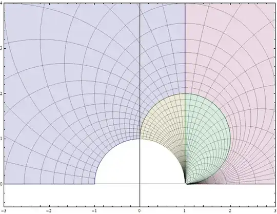
With[{f = Function[z, (z + I)/(z - I)],
      zmin = -(1 + I), zmax = (1 + I)},
      grid = DrawCartesianMap[z, {z, 0, 2 zmax}, Mesh -> {12, 12}, 
             PlotPoints -> 60, MaxRecursion -> 5, 
             BoundaryStyle -> Directive[Thick, Black, Dashed], 
             MeshStyle -> {{Thickness[0.0065], HTML@DarkGreen}, 
                           {Thickness[0.0065], Darker@Brown}}];
      domainObjects = {Opacity[0.5, HTML@Wheat], grid};
      imageObjects = ComplexMap[f][domainObjects];
      Row[{
           Draw2D[{domainObjects}, 
                  PlotRange -> ComplexPlotRange[0.5 zmin, 2 zmax], Frame -> True, 
                  PlotLabel -> z, ImageSize -> Scaled[0.3], BaseStyle -> 12],
           Draw2D[{Arrowheads[.3], NeedhamMappingSymbol[0, 1]},
                   PlotRange -> All, ImageSize -> Scaled[0.05]],
           Draw2D[{imageObjects}, 
                   PlotRange -> ComplexPlotRange[-5 - I, 5 zmax], Frame -> True, 
                   PlotLabel -> f[z], ImageSize -> Scaled[0.3], BaseStyle -> 12]
          },
          Spacer[5], ImageSize -> 720]
    ]

enter image description here

murray
  • 11,888
  • 2
  • 26
  • 50
  • The SE uploader isn't fixed yet, but you can always upload images "old school" style — save as png and use the upload image button in the post editor – rm -rf May 04 '13 at 15:46
  • @rm -rf: As you can see, I did manage to upload a png now. I had completely forgotten about the image uploader built into the editor window. – murray May 04 '13 at 21:47
  • 2
    I fully understand how that must be... I too have gotten quite used to the uploader and grumble when I have to take the long route :) – rm -rf May 04 '13 at 22:41