How can PixelConstrained be emulated with DensityHistogram?

Question

This DensityHistogram doesn't display very well. Some bins are shown much larger than others and, oddly, empty bins appear to be drawn smaller than occupied bins.

DensityHistogram[RandomVariate[BinormalDistribution[.5], 50000], {100, 100}]

enter image description here

In ArrayPlot, similar problems are solved with PixelConstrained. How can PixelConstrained be emulated with DensityHistogram?

I don't understand: what parts of this graphic display "empty bins"? And how are we to tell that bin sizes differ? (Unfortunately your example is not reproducible because you haven't specified a seed--and it takes a bit of time to compute, anyway. Could you offer a simple example of the problem?) I wonder whether you're not just noting aliasing at this resolution. — whuber, Mar 08 '13 at 19:51
@whuber No, I could reproduce it — the pixel sizes indeed are different (try exporting it as a pdf — it's more obvious there). The empty bins that he's talking about are the "white" parts. — rm -rf, Mar 08 '13 at 20:17
@rm-rf I cannot reproduce this behavior even using the command as given (MMA 8.0). When I make the histogram large enough to be able to inspect the "empty bins," I find them to be of the correct sizes. Even when I make it very small, to the degree I can discern any details, I still do not see uneven sizes. (Exporting to PDF adds an unnecessary complication--if the result appears wrong, it could be a problem with the export or with the PDF rendering itself, so I didn't bother to look at that.) — whuber, Mar 08 '13 at 20:41
@whuber Here's a screenshot from my session. Please zoom in well into the region I've marked. You'll see that the squares are all of different sizes. — rm -rf, Mar 08 '13 at 21:03
@rm-rf I really don't see it, nor is it visible in the underlying code. Try Cases[DensityHistogram[ RandomVariate[BinormalDistribution[.5], 50000], {100, 100}], RectangleBox[a___] :> EuclideanDistance@a, Infinity] // Union to see what the kinds of rectangle sizes are present in the plot. They are all virtually the same. I must assume what you see is some kind of aliasing with the pixel raster of your screen. — Sjoerd C. de Vries, Mar 08 '13 at 21:35
@SjoerdC.deVries This is not an issue with the underlying code... only with the display (see my screenshot above), which is fixed with PixelConstrained — rm -rf, Mar 08 '13 at 21:37
@rm-rf I have been measuring an enlarged screendump of my own screen in Photoshop now. There seem to be rectangle size fluctuations in the order of a percent or so. Still hardly noticeable in my opinion. — Sjoerd C. de Vries, Mar 08 '13 at 21:52
@SjoerdC.deVries I agree that one has to go looking for it to actually see it, but it's also one of those things that if you happen to observe it, it's hard to not notice it again. I don't know if it's more noticeable in my case because I have a retina MBP (high pixel density) and mma is not optimized for it. — rm -rf, Mar 08 '13 at 21:55
@rm-rf My image does not look like yours: evidently the squares in your image are all a little too large; the apparent sizes depend on the drawing order. If you're using MMA 9 you should consider reporting this as a bug. — whuber, Mar 08 '13 at 21:56
Skeptics, you're overthinking it. Just look at the image in my question. Compare the size of an isolated purple box to that of an isolated white box. They are very clearly different and the cause of this difference, be it aliasing or something else, is not the subject of the question. The subject of the question is a solution that makes the bins display with identical size by prescribing their size in pixels. — ArgentoSapiens, Mar 08 '13 at 22:27
There may be a solution in the (newer) related question at http://mathematica.stackexchange.com/questions/22527/precision-of-rendered-rectangles-in-stiff-scale-graphics (currently it's only in the comment thread to the question): use Antialiasing -> True. — whuber, Apr 03 '13 at 21:49

score 6 · Accepted Answer · answered Mar 08 '13 at 20:21

I don't quite think you can emulate this with DensityHistogram, but since all it does is computing the 2D histogram and plotting it, we could do those steps ourselves and use ArrayPlot with its nice PixelConstrained option.

Here's a proof of concept:

SeedRandom[1];
data = RandomVariate[BinormalDistribution[.5], 50000];
{bins, counts} = HistogramList[data, {100, 100}];

ArrayPlot[counts, DataReversed -> True, 
    DataRange -> (Through[{Min, Max}@#] & /@ bins), 
    FrameTicks -> {True, True, False, False}, ImageSize -> 500,
    ColorFunction -> "LakeColors", ColorRules -> {0 -> White}, 
    PixelConstrained -> True, Frame -> True, PlotRange -> {{-4, 4}, {-4, 4}}
]

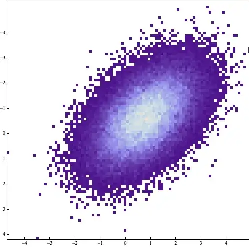
Note that you still need to get the data reversal right and the ticks going the right way to mimic DensityHistogram exactly, but that's a minor detail and I'll leave that to you.

How can PixelConstrained be emulated with DensityHistogram?

1 Answers1

Linked