Let me show how to roll your own numerical solution to a non-linear integral equation using a collocation method. It's fun!
This will involve two approximations. First, we will approximate the function B[x] by its values at n particular points in the range {x, 0, 1}. The integral over x will be replaced by a weighted sum over n, i.e., a quadrature rule. Second, we will only exactly satisfy the integral equation at those n points. It will hopefully be approximately satisfied at other points.
Quadrature rule
Let's borrow one of NIntegrate's quadrature rules:
order = 5;
{abscissae, weights, errweights} =
 NIntegrate`GaussKronrodRuleData[order, MachinePrecision]

The first part abscissae is the list of n points in the range {0, 1} at which we will approximate the solution. The second part weights is the vector of weights for function values at those points to compute an integral estimate.
n = Length[abscissae]

Approximate integral equation
Using the weights of the quadrature rule we can define the approximate integral equation at a single point:
integralEquation[vals_, v_, fv_] := -1 +
  weights.Table[fx v/(fx + fv)^2, {fx, vals}]
Here vals is the list of function values at the abscissae, representing the function B[x] in your question, and v and fv are particular values of v and B[v] in your question.
The value of the above function is zero when the integral equation is approximately satisfied at the specified point.
Here is a vector-valued version that evaluates the approximate integral equation at all of the abscissae:
integralEquation[vals_] :=
 MapThread[integralEquation[vals, ##] &, {abscissae, vals}]
Given the vector of function values at the absissae, it gives the vector of residuals indicating whether the integral equation is satisified:
integralEquation[RandomReal[1, n]]

We would like to find vals such that the residuals are all zero! I.e., we want to find a root of integralEquation.
Find root
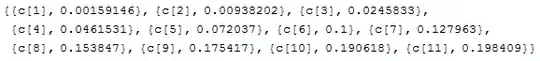
Let's use the symbols {c[1], ..., c[n]} to represent the solved function values at the abscissae:
vars = Array[c, n]

We will find a root using FindRoot, which likes to have a decent guess for the values of the c[i] to start with. By experimenting a little I learned that a linear solution of the form B[x]==0.2*x is a decent guess:
guess = Thread[{vars, 0.2 abscissae}]
Now we can search for a root of integralEquation:
solution = FindRoot[integralEquation[vars], guess]
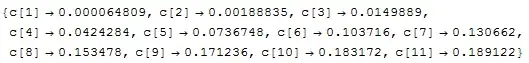
This represents an approximate solution to the integral equation.
Solution function
We can plot the approximate solution over the whole range {0, 1} by interpolating the solution we just obtained at the abscissae:
f[x_] = InterpolatingPolynomial[Thread[{abscissae, vars}] /. solution, x];
Plot[f[x], {x, 0, 1}]

The solution is not exactly correct. In fact, for very small values of x, the residual (the amount by which the integral equation is not satisfied) is substantial. Plot the residual for a few values of x:
residual[f_, v_] :=
 Module[{x}, -1 + NIntegrate[f[x] v/(f[x] + f[v])^2, {x, 0, 1}]];
ListLinePlot[Table[{x, residual[f, x]}, {x, 0.01, 1, 0.01}],
 Frame -> True, PlotRange -> All, AxesStyle -> Dashed]

From here you have some options.
- You could increase the value of
n (by increasing the value of order). You may run into issues with working precision (machine precision may not be enough). You could also use a local interpolation (Interpolation) instead of a global interpolation (InterpolatingPolynomial), which might be more stable for large n.
- You might be able to solve the tricky bit near
x==0 with other methods such as a power series expansion.
Here is a notebook containing the above prototype.
Linear integral equation
For the benefit of people solving related problems, let me just mention that we used FindRoot to search for a root (starting from a plausible guess) because this is a nonlinear integral equation. For a linear integral equation, you can use the same collocation method, but the integralEquations will be linear, so you can be sure of finding a solution simply by using Solve, or reformulate as a matrix problem and use LinearSolve.