Equidistant points on a polyline

Question

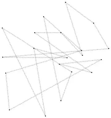
Set of 2D-points connected by a polyline B-spline function:

p = RandomReal[{-1, 1}, {20, 2}];
f = BSplineFunction[p,
   SplineDegree -> 1,
   SplineClosed -> True];

This is neatly defined polyline function. However, as the spline parameter goes from 0 to 1 with some constant step, calculated points are somewhere denser than at other regions. (I can see the density decreases with distance between points.)

Graphics[{
  Point[p], Opacity[.2],
  Point[f /@ Range[0, 1, .001]]}]

enter image description here

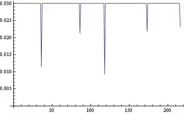
Me I need a function that returns equidistant points for equidistant parameter values.

Graphics[{
  Point[p], Opacity[.2],
  Point[g /@ Range[0, 1, .001]]}]

enter image description here

Where g I constructed like this:

g[t_] := Evaluate[
  With[{u = With[{
       d = EuclideanDistance @@@ Partition[p, 2, 1, 1]},
      Accumulate[d]/Total[d]]},
   Piecewise[Table[{
      p[[i]] + (t - If[i > 1, u[[i - 1]], 0])/
         (u[[i]] - If[i > 1, u[[i - 1]], 0])*
        (p[[If[i != Length@p, i + 1, 1]]] - p[[i]]),
      t <= u[[i]]}, {i, Length@p}]]]]

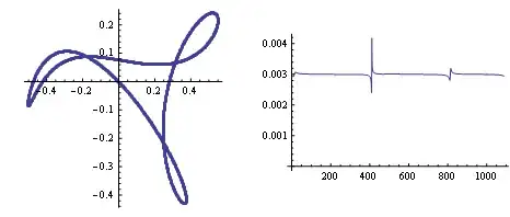
This can be made more elegantly, right, with Mathematica? With some option that samples equidistant points? Because say I have some smooth curve function. I don't know how I would tackle this then. I guess one would have to integrate and findroot some.

Do you actually need the values of the points, or do you just want to connect them with nicely spaced dotted lines? — bill s, Mar 24 '13 at 16:57
Related or duplicate? Generating evenly spaced points on a curve — Vitaliy Kaurov, Mar 24 '13 at 17:15
@bills Values, yes. Otherwise Dashing? :) Vitaliy linked to an elegant solution, will study that. — BoLe, Mar 24 '13 at 18:02

score 11 · Answer 1 · edited Oct 11 '16 at 01:09

You need what is sometimes called a reparametrization by arc length. Since the velocity is piecewise constant, it might done as follows:

p = RandomReal[{-1, 1}, {20, 2}];
f = BSplineFunction[p, SplineDegree -> 1, SplineClosed -> True];
arclengths = Accumulate[Norm /@ Subtract @@@ Partition[p, 2, 1, 1]];
totalarclength = Last[arclengths];
t = Interpolation[
      Transpose@{Prepend[arclengths, 0.], Range[0, 1, 1/Length[p]]},
      InterpolationOrder -> 1];

Graphics[{Point[p], Opacity[.2], 
  Point[(f[t[#]]) & /@ Range[0, totalarclength, totalarclength/1000]]}]

Plot of points

Or one could use calculus to find t as in the link in Vitaliy Kaurov's comment that I just noticed, or in this alternative way:

v[t_?NumericQ] := Norm[f'[t]];
t = NDSolveValue[{tt'[s] == 1/v[tt[s]], tt[0] == 0}, tt, {s, 0, totalarclength}];

Dr. belisarius · Accepted Answer · 2013-03-25T11:34:51.490

p = RandomReal[{-1, 1}, {5, 2}]; 
f = BSplineFunction[p, SplineDegree -> 1, SplineClosed -> True];

A very simple approach:

np[u_, dt_] := u + dt/ Norm[D[f[t], t]] /. t -> u;
ListPlot[Table[f[t], {t, NestWhileList[np[#, .03] &, 0, # < 1 &]}], AspectRatio -> 1]

Mathematica graphics

Testing that the points are equidistant:

ListLinePlot[EuclideanDistance @@@ 
          Partition[Table[f[t], {t, NestWhileList[np[#, .03] &, 0, # < 1 &]}], 2, 1],
          AxesOrigin -> {0, 0}]

Mathematica graphics

The only small exceptions are at the original points, as expected.

Edit

For a higher degree interpolation:

p = RandomReal[{-1, 1}, {7, 2}];
f = BSplineFunction[p, SplineDegree -> 5, SplineClosed -> True]; 
GraphicsRow@{
  ListPlot[Table[f[t], {t, NestWhileList[np[#, .003] &, 0, # < 1 &]}], AspectRatio -> 1], 
  ListLinePlot[EuclideanDistance @@@ 
               Partition[Table[f[t], {t, NestWhileList[np[#, .003] &, 0, # < 1 &]}], 2, 1], 
               AxesOrigin -> {0, 0}, PlotRange -> All]}

Mathematica graphics

Basic-calculus approach, clean and tiny. Thank you. The jumping around the original point parameter values isn't noticeable in my animation -- and I can decrease the step size which diminishes the jumping, and then Take only every second, third or so point since there are probably too many for my purpose. — BoLe, Mar 25 '13 at 12:57

Equidistant points on a polyline

2 Answers2

Linked

Related