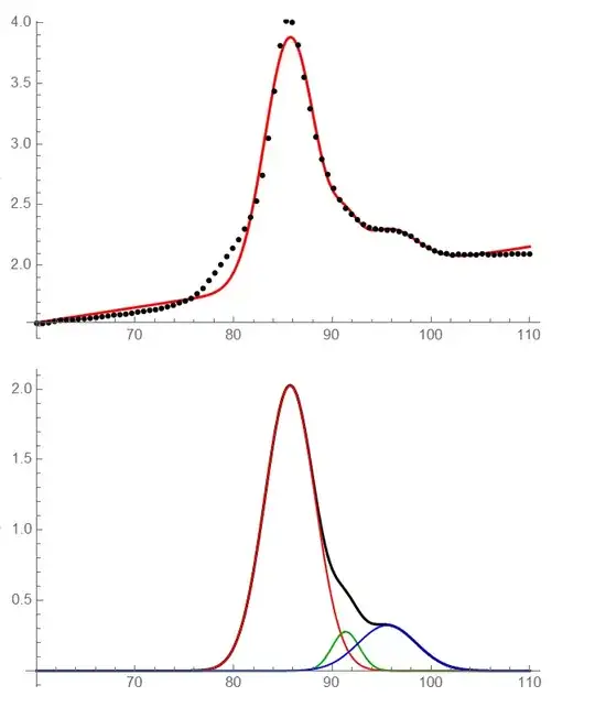
Restrict gaussian multi-peak fitting by area

Question

I am trying to implement the code developed by @MarcoB here: Multi-peak fitting and area of the fitting but trying to restrict the fitting of the peaks by the area, height, the width and the position, rather than only by the height, the width or the position (as it is currently in the code below) in the NonlinearModelFit part of the code. Since I know the maximum area of the last peak (blue) and the middle peak (green), I would like to have an "extra knob" and restrict the NonlinearModelFit with the area as well such as 0 <= area[3] <= "max area of peak" or 0 <= area[2] <= "max area of peak". The maximum area of the 3rd peak (blue) is 1.2 and the one for the second peak (green) is 0.7.

As an example in the code I could restrict the width, height and position as follows:

nlm = NonlinearModelFit[
  peak, {Sum[gaussmodel[height[i], width[i], position[i]], {i, 3}] + 
    slope x + baseline, 0 <= height[1] <= 0.4,84 <= position[1] <= 86.5, 2.9 <= width[1] <= 3.0,
    0 <= height[2] <= 0.3,86.6 <= position[2] <= 93,1.5 <= width[2] <= 1.52, 
   0 <= height[3] <= 0.2,95 <= position[3] <= 98, 2.92 <= width[3] <= 2.93}, {slope, baseline,
    height[1], width[1],position[1], height[2], 
   width[2],position[2], height[3], 
   width[3],position[3]}, x]

But I do not know how to do the same, restricting the NonlinearModelFit by the area of the peaks as well.

Here's the entire code written by @MarcoB (with no restrictions except for the peak position):

data = Import["https://pastebin.com/raw/QCAKwZ2P", "Package"];
ClearAll[gaussmodel]
gaussmodel[height_, width_, position_] := 
 height Exp[-(x - position)^2/(2 width^2)]
peak = Select[data, 60 <= First[#] <= 110 &];
nlm = NonlinearModelFit[peak, 
   Sum[gaussmodel[height[i], width[i], position[i]], {i, 3}] + 
    slope x + baseline, {slope, baseline, height[1], 
    width[1], {position[1], 86}, height[2], 
    width[2], {position[2], 93}, height[3], 
    width[3], {position[3], 96}}, x];
Show[Plot[nlm[x], Evaluate@Flatten@{x, MinMax@peak[[All, 1]]}, 
  PlotStyle -> Directive[Thick, Red]], 
 ListPlot[peak[[;; ;; 10]], PlotStyle -> Black]]
Show[(fitted peak-baseline)
 Plot[nlm[x] - (slope x + baseline) /. nlm["BestFitParameters"], 
  Evaluate@Flatten@{x, MinMax@peak[[All, 1]]}, 
  PlotStyle -> Directive[Thick, Black]],(single components)
 MapThread[
  Plot[#1, Evaluate@Flatten@{x, MinMax@peak[[All, 1]]}, 
    PlotStyle -> #2, PlotRange -> All] &, {Table[
    gaussmodel[height[i], width[i], position[i]] /. 
     nlm["BestFitParameters"], {i, 3}], {Red, Darker@Green, Blue}}]]

Which gives for this data:

A gaussmodel of the form height Exp[-(x - position)^2/(2 width^2)] has an area of height* Sqrt[2 \[Pi]]*width. — JimB, Jun 25 '20 at 02:07
@JimB, thank you! This is very helpful. I actually did not know this!. I really appreciate it !!! (+1) — John, Jun 25 '20 at 02:22

score 1 · Accepted Answer · answered Jun 25 '20 at 17:07

As JimB mentioned in comments, it is easy to show that the area of a Gaussian peak is simply proportional to the product of its width and height:

Integrate[
  gaussmodel[height, width, position], {x, -Infinity, Infinity},
  Assumptions -> {height > 0, width > 0, position > 0}
]
(* Out: height Sqrt[2 Pi] width *)

It is straightforward to use that to generate constraints for the model:

nlm = NonlinearModelFit[
  peak,
  {
    Sum[gaussmodel[height[i], width[i], position[i]], {i, 3}] + slope x + baseline,
    1.1 < Sqrt[2 Pi] height[3] width[3] < 1.3,
    0.6 < Sqrt[2 Pi] height[2] width[2] < 0.8
  },
  {slope, baseline,
   height[1], width[1], {position[1], 86},
   height[2], width[2], {position[2], 93},
   height[3], width[3], {position[3], 96}},
  x
];

Using the code in your question from my previous answer, this returns:

The peak areas are:

areas = Table[Sqrt[2 Pi] height[i] width[i], {i, 3}] /. nlm["BestFitParameters"]
(* Out: {13.2893, 0.799987, 1.29999} *)

However, if one combines these with the constraints you had added about height, width and positions, the fit becomes pretty bad:

nlmJohn = 
 NonlinearModelFit[peak, 
  {
   Sum[gaussmodel[height[i], width[i], position[i]], {i, 3}] + slope x + baseline, 
   0 <= height[1] <= 0.4, 84 <= position[1] <= 86.5, 2.9 <= width[1] <= 3.0, 
   0 <= height[2] <= 0.3, 86.6 <= position[2] <= 93, 1.5 <= width[2] <= 1.52, 
   0 <= height[3] <= 0.2, 95 <= position[3] <= 98, 2.92 <= width[3] <= 2.93, 
   1.1 < Sqrt[2 Pi] height[3] width[3] < 1.3,
   0.6 < Sqrt[2 Pi] height[2] width[2] < 0.8
  },
  {slope, baseline, 
   height[1], width[1], position[1],
   height[2], width[2], position[2],
   height[3], width[3], position[3]},
 x]

The areas in this case are {2.52598, 0.714181, 1.19647}.

At this point, though, you want to re-examine what you are doing. It appears that you either have external information that makes the fitting somewhat redundant, or you pretty much know what answer you want and you are just dressing it up in a cloak of respectability by pretending that it came from a fitting routine. Since your constraints are so strict, it might be easier to use a Manipulate and find the best numbers that fit your results, at least as starting points to a fit.

MarcoB thank you!. I accepted your answer. Also credits to JimB as his comment also pretty much solve the problem as well. — John, Jun 25 '20 at 17:19

Restrict gaussian multi-peak fitting by area

1 Answers1