Color regions defined by many lines

Question

Consider the following code:

 PerpBis[pt1_, pt2_] := 
 Block[{mid = Midpoint[{pt1, pt2}], vec = pt2 - pt1, gamma},
  gamma = -vec[[1]]*mid[[1]] - vec[[2]]*mid[[2]];
  vec[[1]]*x + vec[[2]]*y + gamma == 0
  ]
Show[
 Table[ContourPlot[
   Evaluate@PerpBis[{0, 0}, {i, j}], {x, -5, 5}, {y, -5, 5}], {i, -2, 
   2}, {j, -2, 2}]]

If you run it you will get something like this,:

These line represent Brillouin zones. I would like to highlight each Brillouin zone by colouring its fragmented parts with the same colour. A Brilluin zone is defined by the following statement

• In general, the n-th Brillouin zone consists of the set of points that can be reached from the origin by crossing exactly n − 1 distinct Lines.

In short I want something like this :

Do you have an elegant solution ? I was thinking some Image treatment, some morphological component stuff, the math seems tedious..

Answer 1

Method #1: Image Processing

Find intersections

PerpBis[pt1_, pt2_] := 
 Block[{mid = Midpoint[{pt1, pt2}], vec = pt2 - pt1, gamma}, 
  gamma = -vec[[1]]*mid[[1]] - vec[[2]]*mid[[2]];
  vec[[1]]*x + vec[[2]]*y + gamma == 0]
crossings = 
  Table[{x, y} /. 
    Solve[PerpBis[{0, 0}, {x1, y1}] && 
      PerpBis[{0, 0}, {x2, y2}]], {x1, -2, 2}, {y1, -2, 2}, {x2, -2, 
    2}, {y2, -2, 2}];
crossingsFiltered = 
  Cases[Flatten[crossings, 4], {_?NumericQ, _?NumericQ}] // 
   DeleteDuplicates;

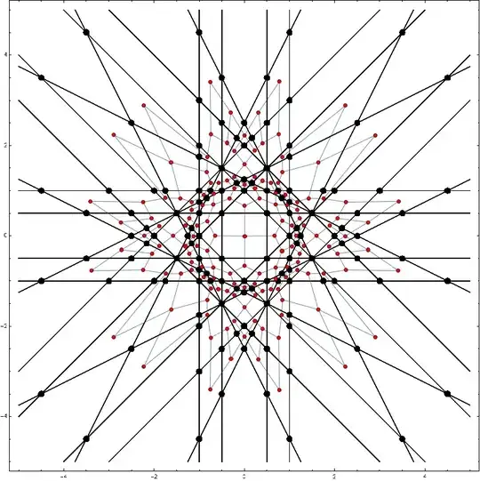
Create two plots

We add line intersections as big black points to the first plot img which will help us determine the neighbouring regions. The second one will be used to produce the final image. Both plots should be created equally so that they concide. ImageSize should be large enough so that even the smallest zones are visible.

out = Show[
   Table[ContourPlot[
     Evaluate@PerpBis[{0, 0}, {i, j}], {x, -5, 5}, {y, -5, 5}, 
     ContourStyle -> Black], {i, -2, 2}, {j, -2, 2}], 
   ListPlot[crossingsFiltered, PlotStyle -> Black, 
    PlotMarkers -> {Automatic, 12}]];
img = Binarize@Rasterize[out, ImageSize -> 800];
plot = Rasterize[
   Show@Table[
     ContourPlot[
      Evaluate@PerpBis[{0, 0}, {i, j}], {x, -5, 5}, {y, -5, 5}, 
      ContourStyle -> Black], {i, -2, 2}, {j, -2, 2}], 
   ImageSize -> 800];
{img, plot} // GraphicsRow

Find Brillouin zones

We use MorphologicalComponents to find the zones. Then Dilation is used so that the lines disappear.

dilationSize = 10;
m = DeleteBorderComponents[
   Dilation[
    DeleteSmallComponents[
     MorphologicalComponents[img, CornerNeighbors -> False], dilationSize], .5],
    CornerNeighbors -> False];
plotComp = 
  DeleteBorderComponents@
   DeleteSmallComponents[
    MorphologicalComponents[Binarize@plot, CornerNeighbors -> False], 
    50];
m // Colorize

Create graph

First, we extract morphological parameters (labels, centroids and neighbors). Because we've added the black points, the neighboring Brillouin zones will be correctly identified.

nodes = ComponentMeasurements[m, "Label", CornerNeighbors -> False][[All, 1]];
centroids = ComponentMeasurements[m, "Centroid", CornerNeighbors -> False];
neighbors = ComponentMeasurements[m, "Neighbors", CornerNeighbors -> False];
g = Graph[nodes, 
   DeleteDuplicates[
    Sort /@ Flatten[
      neighbors /. (i_ -> {l___}) :> (i [UndirectedEdge] # & /@ 

{l})]], VertexCoordinates -> centroids, VertexSize -> .5, 
   VertexStyle -> Red];
Show[img, g]

Calculate distances

The central Brillouin zone corresponds to the center of graph (smallest eccentricity). Then we find a mapping between morphological components of both plots.

centerNode = First@GraphCenter[g];
distance = GraphDistance[g, centerNode];
centroidsRounded = #[[1]] -> Round@#[[2]] & /@ centroids;
plotRules = 
  MapThread[
   plotComp[[-#1[[2, 2]], #1[[2, 1]]]] -> #2 + 1 &, {centroidsRounded,
     distance}];

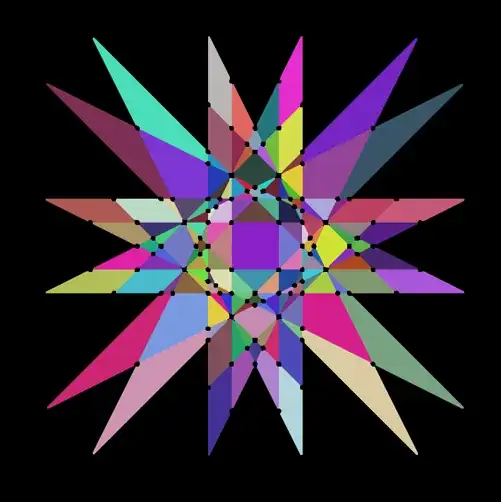
Create plot

First we hide the areas around the Brillouin zones. Then we use some fancy color scheme.

finalPlot = plotComp /. {0 -> -1, 1 -> -1};
finalPlot = 
 ColorReplace[
  Colorize[Replace[finalPlot, plotRules, 2], 
   ColorFunction -> ColorData[93], ColorFunctionScaling -> False], 
  Black -> Transparent]
ImageCompose[plot, finalPlot]

Warning

Because we use image processing, we have to be careful to examine the final results. If the initial image resolution is too small, some zones might get missed. If the intersections are not plotted large enough or dilationSize is too large, some zones may get wrongfully connected as neighbours.

Method #2: Dual Graph

Why bother with image processing when we can calculate the exact positions of all the vertices and edges.

Generate graph

lines = (Table[PerpBis[{0, 0}, {x1, y1}], {x1, -2, 2}, {y1, -2, 2}] //
       FullSimplify // Flatten) /. True -> Nothing;
crossings = ({x, y} /. Solve[#[[1]] && #[[2]]]) & /@ 
   Tuples[lines, {2}];
nodes = Cases[Flatten[crossings, 1], {_?NumericQ, _?NumericQ}] // 
   DeleteDuplicates;
(* Connect neighbouring points on the same line *)
generateEdges[pts_] := Partition[SortBy[pts, nodes[[#]] &], 2, 1];
(* Generate all possible edges *)
edgesAll = 
  Flatten[generateEdges[
      Pick[Range@Length@nodes, 
       Function[p, # /. {x -> p[[1]], y -> p[[2]]}] /@ nodes]] & /@ 
    lines, 1];
(* Remove self-edges and turn lists into undirected edges *)
edges = Select[edgesAll, #[[1]] != #[[2]] &] /. {a_, b_} :> 
     a [UndirectedEdge] b // DeleteDuplicates;
G0 = Graph[Range[Length@nodes], edges, VertexCoordinates -> nodes]

Find dual graph

There seems to be no build-in function to generate a dual graph. So we will generate it ourselves. First, we find faces with IGraph, but this can also be done without any packages. Then, we compare the edges and find the neighbouring faces.

<< IGraphM`
(* Find faces *)
faces0 = IGFaces[G0];
(* Remove the outer-most face *)
faces = Sort[faces0][[1 ;; -2]];
(* Calculate centroids *)
facesCenter = Mean[Part[nodes, #]] & /@ faces;
(* Make the first vertex appear again at the end of the list *)
facesVertices = Append[#, #[[1]]] & /@ faces;
(* Create lists of edges *)
facesEdges = (Sort /@ Partition[#, 2, 1]) & /@ facesVertices;
(* Find faces that share an edge *)
conn = Table[
     If[i < j && 
       Length[facesEdges[[i]] [Intersection] facesEdges[[j]]] == 1, 
      i [UndirectedEdge] j, Nothing], {i, 1, Length@facesEdges}, {j, 
      1, Length@facesEdges}] // Flatten // DeleteDuplicates;
G = Graph[Range@Length@faces, conn, VertexCoordinates -> facesCenter]

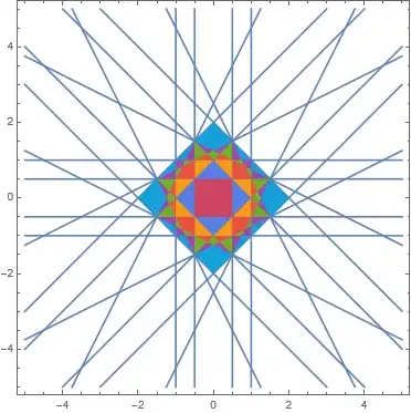
Calculate distances

This is done the same as before. However, let's now take only first few Brillouin zones.

centerNode = First@GraphCenter[G];
distances = GraphDistance[G, centerNode];
(* Maximal Brillouin zone *)
maxDistance = 7;
ind = LessThan[maxDistance] /@ distances;
brillouinZones = 
  Graphics[MapThread[{ColorData[106][#2], 
      Polygon[Part[nodes, #1]]} &, {Pick[facesVertices, ind], 
     Pick[distances, ind]}]];
plot = ContourPlot[Evaluate@#, {x, -5, 5}, {y, -5, 5}] & /@ lines;
Show[plot, brillouinZones]

Advantages

This method has significant advantages over the image processing method because (1) it does not need any manual fine-tuning, (2) it generates polygons instead of a rasterized image, (3) it is certain to correctly find all the zones.

Answer 2

A kludgey implementation that struggles at some of the "points" of the zones:

1. Define a function that takes an equation defining the boundaries and turns it into an inequality satisfied if a point is on the same side of the boundary as the origin is.

   PerpBisIneq[pt1_, pt2_] := Block[{eq = PerpBis[pt1, pt2]},
      If[eq === True, True,
       If[(First[eq] /. {x -> 0, y -> 0}) > 0, Greater @@ eq, 
        Less @@ eq]]
      ]
   

2. Define a function that returns a list of inequalities as functions of the point {x,y}.

   ineqs[{x_, y_}] = 
    Flatten[Table[PerpBisIneq[{0, 0}, {i, j}], {i, -2, 2}, {j, -2, 2}]]
   

3. Create a RegionPlot defined by the region of the plan in which precisely $n-1$ elements of ineqs are False.

   brillouinZone[n_] := RegionPlot[
     Count[ineqs[{x, y}], False] == n - 1, {x, -5, 5}, {y, -5, 5}, 
     PlotStyle -> ColorData[109][n], PlotPoints -> 100]
   

4. Plot the Brillouin zones.

   Show[
     Table[ContourPlot[Evaluate@PerpBis[{0, 0}, {i, j}], {x, -5, 5}, {y, -5, 5}], {i, -2, 2}, {j, -2, 2}], 
     Table[brillouinZone[n], {n, 1, 5}]
   ]
   

A few notes on how this could be refined:

• The equation for i = j = 0 always evaluates as True, requiring the first layer of case-checking in PerpBisIneq. The second layer of case-checking is not necessary if gamma is always negative, but I'm not sure if this is the case.

• The setting for PlotPoints in the definition of BrillouinZone is necessary to get Mathematica to return a "nice" plot. Lower settings cause it to miss some zones entirely.

• There is probably a nicer way of getting Mathematica to logically reduce the condition "precisely $n$ of these inequalities are False" than the way that I've done it, in which Mathematica is (I think) effectively sampling the plane point-wise. I suspect there's a way to do it with Reduce or something similar, but I'm not immediately sure what it is.

• The color scheme can be changed by substituting another number for 109 in the definition of BrillouinZone.

EDIT: I was able to use Reduce to find a set of logical predicates for the nth Brillouin zone. But it's ugly as sin and slow as molasses, so I can't say I recommend it. It might, however, be helpful if you ever need to rigorously define a Brillouin zone (for, say, some kind of integration), so I'm including it for reference.

Brillouinpred[{x_, y_}, n_] := 
 Reduce[Or @@ Apply[And, Subsets[ineqs[{x,y}],{Length[ineqs[{x, y}]] - (n + 1)}], {1}] && 
     ! (Or @@ Apply[And, Subsets[ineqs[{x,y}], {Length[ineqs[{x, y}]] - n}], {1}])]

This returns a logical condition on x and y which is True if {x,y} is in the nth Brillouin zone and False otherwise. This is done by noting that if we have a set of $N$ predicates $P = \{P_1, P_2, ..., P_N\}$, then the statement that "no more than $m$ of the predicates are true" is equivalent to $$ \mathcal{P}_m = \bigvee_{Q \subset P,\, |Q| = N-m} \left[ \bigwedge_{P_i \in Q} P_i \right]. $$ The outer "or" runs over all subsets of cardinality $N-m$, and the inner "and" runs over the elements of each such subset. One can then construct the predicate "exactly $m$ predicates are true" by demanding that $\mathcal{P}_m \wedge \neg \mathcal{P}_{m-1}$. The code above explicitly constructs this statement and then applies Reduce to it for simplification purposes. However, note that this creates a set of ${N \choose m}$ logical predicates, each containing $N-m$ subpredicates, as an intermediate step; so Mathematica takes some time to solve this.

Answer 3

Here is a little generalization of Micheal's answer for anyone wanting to plot 3D Brillouin zones for arbitrary lattices, it is slow as hell, and not commented but as I said it is a generalization of Micheal's answer (the 3D thing works in mathematica 12 but not 11.3...)

    pbp[{0, 0, 0}, r_] = True;
pbp[{0, 0}, r_] = True;
pbp[{0., 0., 0.}, r_] = True;
pbp[{0., 0.}, r_] = True;
pbp[v_, r_] := v.r/v.v <= 1/2 (*The half space below vector v *)
equiDistantPoints[list_] := Reverse@Values[GroupBy[list, Norm]];
lim = 7;
pointList2D = 
  Flatten[Table[{i, j}, {i, -lim, lim}, {j, -lim, lim}], 1];
orderedPointList2D = equiDistantPoints[pointList2D];
pointList3D = 
  Flatten[Table[{i, j, k}, {i, -lim, lim}, {j, -lim, lim}, {k, -lim, 
     lim}], 2];
orderedPointList3D = equiDistantPoints[pointList3D];
WS2D[n_, B_] := 
 FullSimplify[
  Flatten[Table[
    pbp[{point[[1]], point[[2]]}.B, {x, y}], {point, 
     orderedPointList2D[[n]]}]]]
WS3D[n_, B_] := 
 FullSimplify[
  Flatten[Table[
    pbp[{point[[1]], point[[2]], point[[3]]}.B, {x, y, z}], {point, 
     orderedPointList3D[[n]]}]]]
Eq2D[a1_, a2_, n_] := 
 Block[{B = {{-a2[[2]], a2[[1]]}, {-a1[[2]], a1[[1]]}}, newPointList, 
   equations},
  B[[1]] = (2 [Pi]B[[1]])/(B[[1]].a1);
  B[[2]] = (2 [Pi]B[[2]])/(B[[2]].a2);
  newPointList = pointList2D.B;
  equations = Flatten@Table[WS2D[i, B], {i, n}]
  ]
Eq3D[a1_, a2_, a3_, n_] := 
 Block[{B = {a2[Cross]a3, a3[Cross]a1, a1 [Cross] a2}, 
   newPointList, equations},
  B[[1]] = (2 [Pi]B[[1]])/(B[[1]].a1);
  B[[2]] = (2 [Pi]B[[2]])/(B[[2]].a2);
  B[[3]] = (2 [Pi]B[[3]])/(B[[3]].a3);
  newPointList = pointList3D.B;
  equations = Flatten@Table[WS3D[i, B], {i, n}]
  ]
PerpBis[pt1_, pt2_] := 
 Block[{mid = (pt1 + pt2)/2, vec = pt2 - pt1, gamma},
  gamma = -vec[[1]]mid[[1]] - vec[[2]]mid[[2]];
  vec[[1]]x + vec[[2]]*y + gamma == 0
  ]
brillouinZone2D[a1_, a2_, npts_, n_] := 
 Block[{ineqs = Eq2D[a1, a2, npts]},
RegionPlot[
   Count[Evaluate@ineqs, False] == n - 1, {x, -10, 10}, {y, -10, 10}, 
   PlotStyle -> ColorData[109][n], PlotPoints -> 100]]
brillouinZone3D[a1_, a2_, a3_, npts_, n_] := 
 Block[{ineqs = Eq3D[a1, a2, a3, npts]},
RegionPlot3D[
   Count[Evaluate@ineqs, False] == n - 1, {x, -20, 20}, {y, -20, 
    20}, {z, -20, 20}, PlotPoints -> 100]
  ]
Show[Table[brillouinZone2D[{1, 0}, {0, 1}, 7, n], {n, 1, 5}]]
 Show[Table[brillouinZone2D[{1, 0}, {0, 1}, 7, n], {n, 1, 5}]]

 Show[brillouinZone3D[{1, 0, 0}, {0, 1, 0}, {0, 0, 1}, 7, 3]]